Unsupervised and Semi-supervised Learning; An Overview
Contributors: Alice RuedaAndrey MelnikJiri StodulkaJonathan MikkilaRafik GouiaaRogelio CuevasTryambak KaushikWilly Rempel
Editors: Chris BobotsisSusan Shu Chang
This blog post is the collective work of the participants of the Deep Learning Without Labels workshop organized by Aggregate Intellect. This post serves as a proof of work, and covers some of the concepts covered in the workshop in addition to advanced concepts pursued by students.
Table of Contents
Introduction
Author: Willy Rempel| Author | Contribution |
|---|---|
| Willy Rempel |
Introduction
Unsupervised learning has the advantage of being universally applicable whether labelled data is available or not. It can also be used in conjunction with supervised methods in order to squeeze out even more utility from the data. For example, if only a few labelled data points are available, then it may be possible to use unsupervised techniques to come up with a decision boundary to further categorize and label any remaining data. Additionally, data-augmentation techniques can be used to synthetically generate additional training data from the original set.
Data compression is already a form of unsupervised learning. PCA (principal component analysis) and autoencoders (AE) are both examples of this. AEs, though, have the additional benefit of learning non-linear manifolds that PCA cannot do. Additionally, autoencoders can be used for tasks such as: image denoising [1], image in-painting [2], context encoding [3], and semantic hashing [4].
Generative deep models are another set of options. Variational autoencoders modify the original AE by replacing the latent layer (effectively a codebook), with a set of gaussian’s (one vector for the means, another for the variances). The loss function for VAE, referred to as ‘evidence lower bound’ (ELBO), includes a KL-divergence term as a regularizer. This term aids in generating samples at the expense of clustering. A variant, Beta-VAE, amplifies this term which results in ‘feature disentangling’. Disentangling means that each latent dimension will tend to encode for only one independent feature of the data.
GANs are another unsupervised generative model which are quite popular and have been well covered in the literature and online. A final example of unsupervised learning is Word2Vec (skip-gram) used in natural language processing (NLP). Generative models have the advantage of learning a meaningful representation of the data, and can be used to generate additional new data. They also generally perform better than non-generative models such as AE. This comes at the cost of increased complexity and difficulty in training (both convergence and in cost).
Clustering techniques are another way to inexpensively extract as much value from the data as possible. Clustering requires both a proximity measure and a criteria to determine cluster membership. Two common clustering methods from traditional machine learning is K-Means and Expectation-Maximization (EM).
For deep clustering there are several algorithms available. VaDE (Variational Deep Embedding) modifies a VAE with the inclusion of a gaussian mixture model (GMM). Instead of sampling directly from the latent variable , first a category variable is sampled from the GMM which conditions the sampling of . The sampling of is from a learned distribution , and the parameters of the mixture model are learned prior to training the VAE model. Other deep clustering techniques include: deep adversarial clustering (DAC) [5], deep embedded clustering (DEC) [6], CatGAN [7], InfoGAN [8], and for a non-parametric technique, deep belief networks (DBN) [9]. For time series, PredNet is a generative RNN (recurrent) model which predicts the next data point () and forwards the error as input to the next layer (). PredNet has the advantage of unsupervised learning of entire scenes but is computationally intensive and prone to blurry reconstruction.
For deep clustering performance metrics we have 3 options available:
-
Unsupervised clustering accuracy (ACC) which matches clusters to labels (similar to classification)
-
Normalized mutual information (NMI), a measure of correlation between two disjoint clusters
-
Adjusted Rand Index (ARI) which uses pairwise measures within and between clusters
On the positive side, deep clustering gives us both clustering and generation. It also can disentangle features and facilitates visualization. On the negative side it does not initialize well and often needs pre-trained models. It also shares with deep learning in general the added complexity and cost of implementation.
Semi-supervised (or weak) learning, situated between unsupervised and supervised, covers a suite of tools and techniques that practitioners can use to manage data labels (or the lack thereof). Labelled data can be expensive or simply impossible to get. Further labelling problems include labels that are: subjective (ie. how difficult was the test), ambiguous (unclear category), erroneous, partly missing, coarsely estimated (ie. about 5cm long), or unstructured (ie. complex image with many applicable labels).
Self training is a creative approach where we can effectively get labels for free. This is accomplished by transforming the data in some way. For example, colorization takes colour input images, creates another dataset by converting the images to greyscale, and then trains a model to predict the colour of pixels in the images. The labels are the true colour values. Another technique is Jigsaw. Here a section of an image is divided into a grid of disjoint patches and a model is trained to learn the correct relative positions of each patch with respect to the others. Exemplar Networks start by treating each original image as a ‘seed’ image, which also effectively becomes a category. A variety of transformations are performed on the image and then a model is trained to correctly classify each processed image as coming from the original seed image.
Multi Instance Learning (MIL) breaks up the data into subsets, called bags, and applies only one label to the bag instead of every instance. An example where this is useful is with very large medical imaging which cannot be feasibly used as a whole. The image can be decomposed into appropriate sized patches which are put into bags. If one or more of the images are cancerous, then the bag is labelled ‘unhealthy’, otherwise it is ‘healthy’. In this way the model will learn features for healthy and express uncertainty when there is potential cancer. With MIL Pooling we aggregate the scores of all the bag instances in some way to determine the bag label. Attention MIL Pooling is one approach where an additional attention network learns the aggregation function based on the contribution of each instance to the bag label. MIL is useful when the labels are noisy or costly, and also for tasks such as zero and few shot learning.
With pseudo-labelling methods we look for creative ways to infer or augment labels from the data. For example, after a model has been trained on labelled data it can then be used to predict any unlabelled data. Predictions with high scores can then be given pseudo-labels where we cannot be certain but have some confidence that these new labels are correct. The model can then be retrained with both datasets combined. Additionally, uncertain predictions with low softmax scores can be binned separately for human review and correction. This is called active learning and can greatly reduce the amount of costly manual labour required to label a dataset.
The MixUp algorithm creates pseudo-labels as above, but it also keeps a record of all the softmax output scores. At the end of the labelling task the past scores are used to update the pseudo-labels, increasing the confidence of the labelling. A regularizer is also used which increases label confidence as the model is increasingly trained. Co-training uses two networks that are trained simultaneously to correct each other. The aim is for them to agree on correct predictions and disagree on errors. Two networks are used again in Co-teaching where the instances with small losses are fed into the second network. In effect the first network acts as a sort of filter to admit only higher quality labelled data.
Labels can also be directly created by embodying various heuristics into functions that will generate labels for a dataset, such as is done with the Snorkel package. Lastly online and multi-task learning can also be used. For multi-task learning a model can be trained on tasks and datasets which are more accessible and are sufficiently related to the actual task of concern.
In this article, we first present ‘Training Deep Neural Networks on Noisy Labels with Bootstrapping’ which manages noisey labels by a consistency measure. We then move on to ‘RAD: On-line Anomaly Detection for Highly Unreliable Data’. The RAD framework is introduced along with three variants which are assessed. Lastly we look at ‘Cost-Effective Active Learning for Deep Image Classification’ which combines active learning with pseudo-labelling to maximize resource utilization.
References
[1] Denoising Adversarial Autoencoders, Creswell and Bharath, https://arxiv.org/pdf/1703.01220.pdf
[2] Semantic Image Inpainting with Deep Generative Models, Yeh et al, CVPR 2017
[3] Context Encoders: Feature Learning by Inpainting, Pathak et al, CVPR 2016
[4] Semantic Hashing, https://www.cs.utoronto.ca/~rsalakhu/papers/semantic_final.pdf
[5] W. Harchaoui, P. A. Mattei, and C. Bouveyron, “Deep adversarial Gaussian mixture auto-encoder for clustering” in Proc. ICLR, 2017, pp. 1–5.
[6] J. Xie, R. Girshick, and A. Farhadi, “Unsupervised deep embedding for clustering analysis” in Proc. Int. Conf. Mach. Learn., 2016, pp. 478–487.
[7] J. T. Springenberg. (2015). “Unsupervised and semi-supervised learning with categorical generative adversarial networks.” [Online]. Available: https://arxiv.org/abs/1511.06390
[8] X. Chen, Y. Duan, R. Houthooft, J. Schulman, I. Sutskever, and P. Abbeel, “InfoGAN: Interpretable representation learning by information maximizing generative adversarial nets” in Proc. Adv. Neural Inf. Process. Syst., 2016, pp. 2172–2180.
[9] H. Lee, R. Grosse, R. Ranganath, and A. Y. Ng, “Convolutional deep belief networks for scalable unsupervised learning of hierarchical representations” in Proc. 26th Annu. Int. Conf. Mach. Learn., 2009, pp. 609–616.
Training Deep Neural Networks on Noisy Labels with Bootstrapping
Author: Tryambak KaushikAuthor: Jiri StodulkaAuthor: Andrey Melnik| Author | Contribution |
|---|---|
| Tryambak Kaushik | TK contributed to the technical part. |
| Jiri Stodulka | Jiri modified the formatting and conclusions. |
| Andrey Melnik | Andrey typed in LaTeX formulae |
Introduction
Supervised learning and unsupervised learning are two popularly used machine learning (ML) methods. Supervised ML models use dataset labels to train while no labels are used for unsupervised ML models. However, increasingly large and complex datasets can have missing labels and/or incomplete labels. Furthermore, the label of datasets can themselves be biased due to subjective labelling. One of the methods to work with noisy data is to bootstrap the prediction function with notion of a “consistency” [Scott et al. (2015)], by measuring the noise of different predictions from the trained ML model. The authors evaluate consistency based on the similarities in features learned from the deep network, i.e. the network exploits implicit similarities between data samples to categorize them.
The authors successfully use this method to train the “corrupted” MNIST dataset, “subjectively labelled” Toronto Face Database, and “partially labelled” single-shot person detection in the ILSVRC2014 dataset. Here, a “partially labelled” dataset is one which, due to the large dataset volume, does not have all objects annotated.
The authors propose 2 methods to measure consistency:
-
Reconstruction is an explicit method and directly measures the consistency error or noise distribution of model prediction against training labels. The reconstruction used is
where the first term is a weighted log-likelihood loss and the second term is a regularisation term. Here is the data, are the observed multinomial labels for classes, are weights and is the true label for . Finally, is a trade-off parameter and is usually found by cross-validation.
This method becomes difficult to train, however, for complex and high dimensional distributions.
-
Bootstrapping. In this method, the noise is implicitly bootstrapped (or made “self-aware”) to the training labels by using model predictions to generate the training targets. Hence, this method does not directly measure the noise error.
This procedure implicitly relies on of noisy labels to be “inconsistent” by nature, and thus get weeded out as the model learns more consistent features of the dataset. The authors use two bootstrapping models:
-
A “soft” bootstrapping loss function for each batch, defined as:
where is the vector of predicted class probabilities.
-
A “hard” bootstrapping loss function, which instead estimates the maximum value of for a given to evaluate a modified loss function.
This method is particularly useful for weakly linked datasets, i.e., where user behaviours are tend to be exclusive and modelling all output pairs is neither useful nor practical.
-
Similarly, for training on the ILSVRC2014 dataset, the authors modify the Multibox loss function to
and
Here, are training targets and are confidence scores (set to threshold of 0.5 for the hard case) for each of the locations. The indicator has value one if is true, and zero otherwise.
Result
The Reconstruction and Bootstrap loss functions gave consistently higher classification accuracy when the fraction of contaminated data exceeded 38% (Figure 1). Furthermore, it appears that the bootstrap-hard and bootstrap-recon performance is nearly equivalent and can be useful for cases where reconstruction is difficult due to a complex and high dimensional dataset.
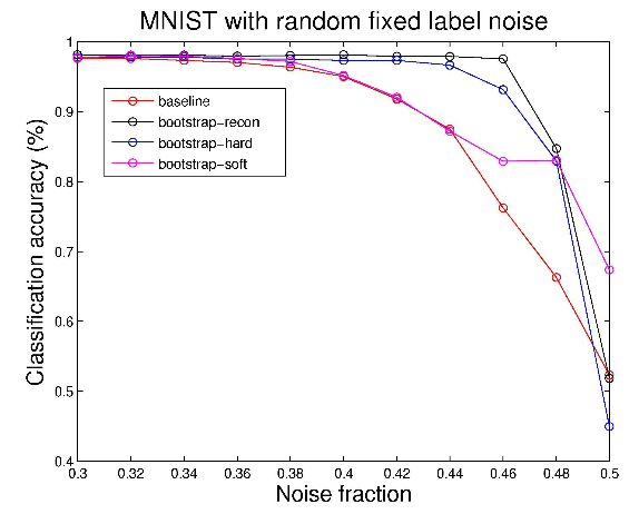
Figure 1. Results of training on MNIST dataset
Similar results were observed for the Toronto Face Database, where bootstrap-recon and bootstrap-hardpredicted with nearly the same accuracy. The improvement in accuracy for all three methods on the TFD dataset suggests that the approach is useful not only for mistaken labels but also for missing labels.
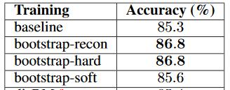
Figure 2. Emotion recognition results on Toronto Faces Database
The precision-recall curve improves significantly for the ILSVRC dataset (Figure 3). It may be noted that bootstrap-hard performs marginally better at high precision while the top-k heuristic performs better at high recall. Top-k heuristic modelling is based on the top k largest confidence predictions being dropped from the loss, i.e., no gradient comes from top k most confident location predictions [Szegedy et al, 2014]. Hence, only the top k most confident locations modify targets to become predictions themselves.
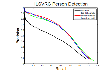
Figure 3. Precision-recall curves compared to baseline-prediction only network and top-k heuristic
Conclusion
The reconstruction and bootstrap methods help improve the performance of ML models on unlabelled and subjectively labelled datasets. Furthermore, it is also demonstrated that with little engineering on loss functions, an accurate performance can be achieved in spite of mistaken labels.
RAD: On-line Anomaly Detection for Highly Unreliable Data
Author: Alice RuedaAuthor: Jonathan Mikkila| Author | Contribution |
|---|---|
| Alice Rueda | Introduction and model sections. |
| Jonathan Mikkila | Results and conclusion sections. |
Introduction
Robust Anomaly Detection (RAD) is a generic framework previously proposed by the authors in [Zhao2019]. The current paper proposed three modified/variational models. These RAD variational models are designed for online anomaly detection on noisy data with wrong labels and continuous learning from the new data.
The models were tested with: (1) 10 classes of IoT attacks; (2) predicting 4 classes of task failures of big data processing cluster; and (3) recognising 20 celebrities’ faces.
Model
RAD is a generic learning framework for continuous online anomaly detection. RAD contains 2 layers. The first layer contains a Label Quality Predictor (L) which performs filtering on suspicious/noisy data. The second layer contains an Anomaly Classification (C) which detects anomaly patterns.
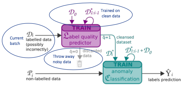
Figure 1. Generic RAD framework with a label quality predictor (L) to determine whether the data is clean (q=1) or not (q=0). Dirty data gets thrown away and clean data will be passed to the anomaly classification (C).
Three variations were presented in the paper: RAD voting, RAD active learning, and RAD slimmed. The three variations are modifications of their predecessor.
-
RAD Voting: In addition to have the label quality predictor (L) determining if the data is noisy or not, anomaly classification (C) will also perform label quality prediction on uncertain data that L determined as noisy. The uncertain data will be either 1) Considered as clean if the classifying result from C is the same as the given label, or 2) the class determined by the L is the same as the class determined by C.
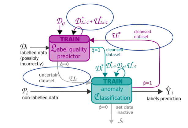
Figure 2. RAD Voting: Instead of throwing away the dirty data, the data is marked as uncertain (U) by L. The uncertain data will be confirmed by C as agreeable data if: 1) the given label is the same as the label determined by C; or 2) Labels determined by AC is the same as L. New labels for the agreeable data follow the labels given by AC.
-
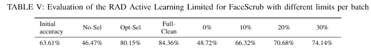
RAD Active Learning: In addition to L and C, the active learning model contains an Oracle, which can correct the labels on the noisy data. The cleansed data can then be used to train the model. The percentage of cleaning can affect the accuracy of the detection. There is also an optional restriction on limiting the number that RAD Active Learning can ask the Expert/Oracle for a true label per batch.
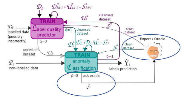
Figure 3. RAD Active Learning: Non-agreeable data from the active learning can also be used with the introduction of an expert system or a person to provide the true label for training
-
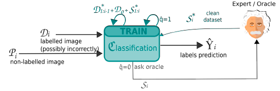
RAD Slimmed: The slimmed version delegates the filtering to the Oracle and eliminates the need of L. If the class prediction from C is different to the label, the data is sent to the Oracle for cleaning. The cleansed data is then used for training.
caption(~Figure 4~, ~RAD Slimmed: Instead of the combined L+C model as in the previous variations, there is only a classifier to simplify the model complexity. Any uncertain data is sent to the oracle for cleaning.~) }}
In the paper, noise was added to the labels with a Gaussian distribution. The paper tested the noise level from 0% to 100%, with a standard deviation (std) of 20%. For a batch of 400 data points, 10% mean-noise level with 20% std affects data points, as in . The labels on the affected data point were replaced by other class labels randomly selected in a uniform distribution.
Results: (use cases)
Task-appropriate results were reported for RAD variants relative to experimental baselines. Beyond the experimental baselines of No-Sel (No RAD) and Opt-Sel (perfectly clean data), typical performance was that for highly contaminated data (noise as high as 30% and 40%) RAD enabled the machine learning models in question to very closely track the performance achieved with reference data uncontaminated by any noise. Whereas for these same noise levels, performance without RAD facilitated corrective feedback was often at or well below the performance at the end of the first batch of training data (Batch #0 in figures to follow). The paper demonstrated that persisting with training with data corrupted by moderate to high noise labels resulted in either failure to realise gains or a dramatic decrease in performance. This further highlights the utility of RAD.
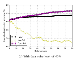
Figures 6A & 7B. RAD performance for IoT -Thermostat and HPC Cluster Task datasets, with noise levels of 30% and 40% respectively.
Beyond simply being corrective for label noise, in specific cases, there was evidence of noise-enhanced learning With RAD enabled learning of noisy data generalizing to a higher degree of accuracy in fewer batches/epochs when compared against training against perfectly clean data. This effect was present at multiple noise levels, but does appear to be task and model specific. This was a very unexpected result.
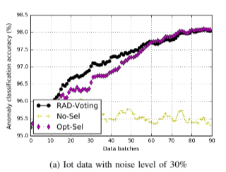
Figures 10A and 11A. IoT and HPC Cluster Tasks dataset classification performance, respectively. Clearly evident in 10A is performance superior to Opt-Sel baseline for much of the training process, and absent from figure 11A. Error bars are plotted on these figures. Please see Figure 10B in the paper for another example of this phenomenon for the dataset at an additional noise level.
Some limitations highlighted by the authors were that the two active methods (Rad-Active and Rad-Slimmed) will most likely be inappropriate for real-time applications. A real-time constraint is the need for an immediate response to be provided for online training. In latency-sensitive or compute limited environments RAD may also introduce added requirements that may limit its applicability. Furthermore, it introduces additional model-risk in the form that the classifier may overfit to label model rather than the data.
Conclusion
The paper provides compelling evidence that where appropriate, the ability to incorporate feedback can dramatically improve measurable outcomes for machine learning enabled projects, even when corrective feedback is on a limited scale. Furthermore, it demonstrated that these techniques are robust when both noise levels are high and corrective feedback is limited (Table V).
References
[Zhao2019] Z. Zhao et al., “Robust Anomaly Detection on Unreliable Data,” Proc. - 49th Annu. IEEE/IFIP Int. Conf. Dependable Syst. Networks, DSN 2019, pp. 630–637, 2019.
Cost-Effective Active Learning for Deep Image Classification
Author: Rafik GouiaaAuthor: Rogelio Cuevas| Author | Contribution |
|---|---|
| Rafik Gouiaa | Equal contribution: summary and code. |
| Rogelio Cuevas | Equal contribution: summary and code. |
I. Context
A common challenge faced during learning-based image classification is the need for a large number of annotated training examples. This poses a considerable downside of such classification methods as labeling data is costly in terms of human effort.
The authors of this paper propose a method that tackles this issue by incorporating active learning within the context of deep learning for image classification.
II. Background
In this section we briefly discuss the two apparently conflicting ingredients that are unified by the authors for their proposed approach: deep learning and active learning.
A. Deep convolutional neural nets for image classification
Deep learning has proven to be a robust and successful method that performs well on classification-related tasks for images. Specifically, convolutional neural networks (CNN) have shown to provide good results as they directly learn features from raw pixels; it learns how to extract features and eventually infers what object the pixels constitute.
CNNs, while successful, have the disadvantage that they require a large number of annotated images. This poses a challenge as annotation of images is expensive not only in terms of time and human effort, due to the expertise needed to do so, but also in terms of the impact a poor annotation can have in sensitive scenarios. An example of this is the annotation of images associated with malignant diseases in patients. Different medical experts may have conflicting opinions in a situation where consensus needs to be reached.
B. Active learning
It is clear that nowadays the volume of data individuals have access to is constantly growing. Making use of it for predictive tasks through modelling, although attractive, poses a great difficulty as the majority of data one can access is not labeled.
The previous difficulty helps make a case for active learning (AL). One aspect behind AL is to improve models that already exist by selecting and annotating unlabeled data samples that show to be most informative. Most informative samples refer to samples where the model is most uncertain and they are found based on three different approaches; such approaches are discussed in Sections III A and III B.
The procedure consists of increasing, in an iterative manner, the size of a previously selected labeled sample. The intention of this procedure is to achieve at least similar performance, if not better, to the one reached when using a fully labeled dataset. Moreover, the cost of performing this iterative process is in principle lower than what it takes to annotate the unlabeled data present in the dataset.
It is important to point out that AL inherently assumes that the feature representation is fixed, which is what allows the possibility of extracting the most informative sample from the original dataset.
In some cases it has been observed that AL methods work by having a model initialized with a small set of labeled data. Then the model is boosted by selecting the most informative samples and sending them to an oracle for annotation. This idea, although promising, faces the problem that the model used for predictions is trained on small datasets and making use of hand-wroughted features.
C. Difficulties in incorporating convolutional neural networks into active learning
The discussion above would suggest that deep learning can benefit from active learning even in the presence of limited labeled data. This is, however, not the case as the AL and DL processes are conflicting. This is due to the fact that, as opposed to CNN, AL extracts the most informative data points relying on the assumption that feature representation is static. This conflict is what motivates the authors to present the approach discussed: cost-effective active learning (CEAL).
III. Cost-effective active learning (CEAL)
In this section we discuss the key idea of CEAL that allows it to avoid the conflict between AL and CNNs mentioned in section II. C. We also discuss previous approaches CEAL improves upon as well as details on how CEAL works and its performance on two datasets.
A. Active learning methods
The main goal of active learning is to make a learning algorithm that is capable of querying an oracle for labels and it choses examples from which to learn the most.
As a result of this, the mechanism which selects the most useful data points is crucial for AL to be successful. There are a few mechanisms that have been explored for this purpose:
- Least confidence. The confidence values are simply the highest class probability score for each example. These values are then ranked, and the lowest valued entries are the ‘least confident’ ones.
- Margin sampling. The smaller the margin sampling value is, the more uncertain an example is. It is computed as the difference of probabilities of an example belonging to either the first or second most probable classes predicted by the classifier.
- Entropy. The larger the entropy is the more uncertain an example is. Entropy is computed as the usual information entropy.
B. The CEAL algorithm
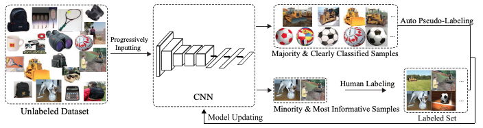
In order to determine the weights of the CNN classifier , CEAL relies on an AL approach that automatically assigns pseudo-labels – labels created with no human intervention - to the unlabelled examples in the dataset. The implementation of this specific AL approach, in combination with a deep CNN, is the key contribution of the authors and what gives rise to CEAL. From now on we denote the dataset of interest as where represents the sample of the dataset and its corresponding label. Each label can take one of the values in the set . This means we have a dataset with n examples and m categories.
The dataset of interest is the union of the set of labeled examples, , and the set of unlabeled examples . That is, . Let us keep in mind that the cardinality of and will change as iterations in CEAL progresses. Initially is the empty set and its cardinality increases gradually as examples from are moved into .
In what follows we explain the steps invoked to learn the optimal value of weights for this CNN.
-
Weights of the deep CNN are initialized to classify a few labeled examples. These labeled examples are obtained from manually annotated examples that have been randomly drawn from.
In addition, one needs to choose an integer number representing the number of iterations, an integer number representing the number informative samples, a real number representing a threshold to identify high confidence samples, which represents the threshold decay rate, and a learning rate based on which the weights of the CNN will be updated. Details and relevance of these parameters will become clear as we present the steps captured by the algorithm.
-
Examples from are fed into the CNN to generate two groups of samples: informative samples and high confidence samples.
Informative samples are chosen based on one of the following criteria:
-
Least confidence. examples with lowest confidence value - the smaller the confidence value is the more uncertain the example is. Confidence value is computed as
-
Margin sampling. examples with lowest margin sampling - the smaller the margin sampling value is the more uncertain the example is. This quantity is computed as
where and represent, respectively, the first and second most probable class predicted by the classifier.
-
Highest entropy. examples with highest entropy value are chosen - the larger the entropy the more uncertain the example is. The entropy of sample , , is computed as
In all three cases just described, represents the probability of belonging to the class.
High confidence samples are chosen as the samples whose entropy is smaller than the threshold . Based on this, the pseudo-label of the example is defined as , where and is the Heaviside function - its value is 1 if the argument is greater than zero and zero otherwise.
Samples with high confidence are captured under a set denoted as .
-
-
Fine tune the CNN by updating the threshold of high confidence samples and its weights based on back propagation. This is achieved by the following iteration. For :
-
Update weights based on learning rate and gradient of the cost function given by
where represents the indicator function and . Notice this implies the first summation is performed over the examples belonging to the union of high confidence samples and labelled samples.
Once this update has been performed, remove pseudo-labels from samples in and put them back into .
-
Update threshold of high confidence as , where ; threshold of high confidence initially chosen by the user.
-
Note that the steps spelled out above implies CEAL has the following hyperparameters:
- number of iterations criteria to choose informative samples;
- number of informative samples ;
- threshold for informative samples;
- threshold decay rate for high confidence samples;
- learning rate to update CNN weights.
The following picture displays, roughly speaking, the CEAL process described in this section.
C. State-of-the-art method compared against CEAL
CEAL is compared with baseline and state-of-the-art methods to provide evidence of its improvement of the existing leading method. The three reference methods are:
-
Active learning all (AL_ALL). All training samples are manually labeled and are used to train CNN. This approach naturally constitutes the upper bound for performance as all data points for training are labelled.
-
Active learning random (AL_RAND). Samples to be labelled are randomly selected to fine-tune the CNN. This approach constitutes a lower bound as active learning techniques are not incorporated.
-
Triple Criteria Active Learning (TCAL). State state-of-the-art active learning method that identifies an effective and small as a possible set of irrelevant and relevant examples based on three criteria: uncertainty and diversity - it selects the most informative examples in the dataset - and density - it selects examples that are representative of the distribution captured in the dataset.
In order to compare CEAL with TCAL, authors prepared a TCAL pipeline by building an SVM classifier and applied uncertainty based on sampling margin strategy, diversity by clustering the most uncertain samples via k-means and density by computing the average distance between a reference data point with other samples within the cluster the reference point belongs to; the point with the smallest average distance (largest density) is the most informative sample.
In the following section we briefly discuss the experiments set to the comparison mentioned as well as the result of such experiments.
D. Datasets, experiments and results
Comparison of CEAL with the three reference methods mentioned in Section III-C was performed on Cross-Age Celebrity face recognition Dataset (CACD) and Caltech-256 object categorization dataset. The former consists of over 160000 images while the latter contains 30607 images of 256 categories. Each dataset was resized and for each of the different parameters of CEAL algorithm were chosen:
- CACD was resized into and the parameters , , , for all layers and .
- Caltech-256 was resized into and the parameters , , , for softmax layer and for all other layers while .
Also, from Section III-B we learned that informative samples can be selected based on three different criteria: least confidence, margin sampling and highest entropy. We denote each of these methods, respectively, CEAL_LC, CEAL_MS and CEAL_EN.
In this section we present the results of different experiments based on different combinations between AL methods against CEAL is compared (AL_RAND, AL_ALL or TCAL) and CEAL selection criteria (CEAL_LC, CEAL_MS or CEAL_EN).
Also, a different experiment is proposed to assess the raw performance of large confidence (LC), margin sampling (MS) and highest entropy (EN) criteria. This experiment consists of disregarding the cost-effective high confidence sample selection step in the algorithm (step 2 of algorithm of Section III-B) and incorporating it into the AL_RAND active learning strategy. This strategy is denoted by the authors as CEAL_RAND. That is, since AL_RAND randomly selects samples to be annotated, CEAL_RAND reflects the original contribution of the pseudo-labeled majority high confidence sample strategies.
All plots below show the classification accuracy for different fractions of annotated samples.
-
CEAL_MS performance. On both datasets CEAL_MS is compared with three AL methods, AL_ALL, AL_RAND and TCAL.
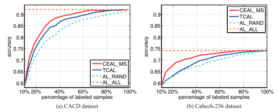
For all fraction of labeled samples, CEAL with margin selection (MS) selection criteria, the graphs suggest that CEAL_MS outperforms AL_RAND and TCAL.
From the numerical values from which these plots are generated, though, it is possible to see that at fractions between 0.7 and 0.8, both CEAL_MS and TCAL are both fairly competitive with AL_ALL and very close to one another in performance. This suggests that the increase in performance offered by CEAL_MS is marginal over TCAL.
-
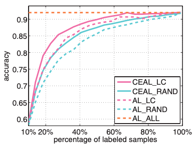
*Least confidence CEAL and AL. CEAL_LC is compared with AL_RAND and AL_ALL active methods on both datasets. Comparison is also done with the respective active learning (in this case least confidence). CEAL_RAND is included as a reference. Panel on the left refers to CACD dataset while the one on the right is for Caltech-256.
-
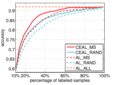
Margin sampling CEAL and AL. Similar to the previous case, CEAL_MS is compared with AL_RAND and AL_ALL active methods on both datasets. Comparison is also done with the respective active learning method (in this case margin sampling). CEAL_RAND is once again included as a reference. Panel on the left refers to CACD dataset while the one on the right is for Caltech-256.
-
Highest entropy CEAL and AL. Similar to the previous case, CEAL_EN is compared with AL_RAND and AL_ALL active methods on both datasets. Comparison is also done with the respective active learning (in this case entropy). CEAL_RAND is once again included as a reference. Panel on the left refers to CACD dataset while the one on the right is for Caltech-256
In experiment 2, 3 and 4 we observe that CEAL when combined with each selection criteria (least confidence, margin sampling and entropy) outperforms active learning combined with the corresponding selection criteria. This improvement, however, seems to be marginal when the fraction of labeled samples get closer to a value between 0.7 and 0.8. This observation is true on both datasets and may suggest that most of the performance is already captured by active learning methods, which would imply that selection criteria has little impact in performance improvement. This is somehow confirmed by the comparison between CEAL_RAND and the active learning method when combined with the corresponding selection criteria.
As a final experiment the authors propose combining CEAL_LC, CEAL_MS and CEAL_EN in the following way. On each iteration of the algorithm, top samples are selected according to each selection criteria, resulting in three sets of data: , and . These three datasets are then combined and duplicates are removed to form the set . Lastly, from random points are taken from it for annotation. This method is denoted by the authors as CEAL_FUSION.
The result of this experiment, in terms of accuracy versus fraction of labeled samples, is shown in the following figure.
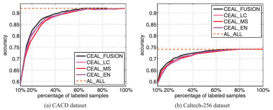
The three different approaches, CEAL_LC, CEAL_MS and CEAL_EN perform similarly for every fraction of labeled samples while CEAL_FUSSION outperforms each of them.
IV. Summary and general comments
The authors propose a way to incorporate active learning into deep learning by selecting informative samples based on three different criteria: least confidence, margin sample and highest entropy. In addition, the authors also propose a mechanism to incorporate high-confidence pseudo-labels.
The approach outperforms state-of-the-art active learning methods in classification tasks when executed in the CACD and Caltech-256 datasets and the ballpark performance is not dramatically sensitive to the selection criteria selected. The improvement is, however, marginal.
One of the advantages of the method is that the number of informative samples needed to reach such performance is a small fraction of the whole dataset - less than 5% in both datasets explored.
The method depends on a number of user-defined parameters to update CNN weights. Although reported, it is not clear how the values chosen for the experiments were selected by the user. An interesting piece of future work would be a study of how sensitive the performance of the method is to the thresholds for informative samples and high confidence samples.
V. Pytorch Implementation:
[Github link]: https://github.com/rafikg/CEALAll the details to use the code is explained in the repo.