Recommender Systems; An Overview
Contributors: Alireza DarbehaniAndrey MelnikChris AlertElham KaramiGurinder GhotraHari RavindranLisa PritchettMadhur KanjoliaMarnie LandonRaul Morales DelgadoRobert HensleySusan Shu ChangTryambak Kaushik
Editors: Susan Shu ChangNick Morrison
This blog post is the collective work of the participants of the Recommender Systems workshop organized by Aggregate Intellect. This post serves as a proof of work, and covers some of the concepts covered in the workshop in addition to advanced concepts pursued by the participants.
Table of Contents
- Introduction
- BERT4Rec: Bidirectional sequential recommendations
- Reinforcement Learning for Slate-based Recommender Systems: A Tractable Decomposition and Practical Methodology
- Deep Learning Recommendation Model for Personalization and Recommendation Systems
- Large-scale Parallel Collaborative Filtering for the Netflix Prize
- Amazon’s item-to-item collaborative filtering
- Pre-training of Context-aware Item Representation for Next Basket Recommendation
Introduction
Author: Susan Shu Chang| Author | Contribution |
|---|---|
| Susan Shu Chang |
Introduction
The workshop first introduced the foundations of recommender systems, such as memory-based and model-based collaborative filtering, elaborated on with the alternating least squares method. Following were methods of ranking evaluation in recommender systems, namely mean average precision and mean reciprocal rank, which provide valuable information on the relevancy of a recommender’s outputs.
Exploring datasets to generate features for recommender systems was also a focus of the workshop: be it user or item features, global features or local features; being able to extract meaningful information from raw data to produce the training set is crucial to building a high performance recommender system. Finally, the workshop covers more advanced techniques such as using variational autoencoders to create latent representations which capture information to produce relevant recommendations.
The following blog post authored by participants of the workshop gives a thorough overview of various topics in recommender systems. These include: BERT4Rec which applies NLP techniques, reinforcement learning in recommender systems, deep learning recommendation model (DLRM), and extensive explanations and applications of various collaborative filtering techniques.
BERT4Rec: Bidirectional sequential recommendations
Author: Robert HensleyAuthor: Madhur KanjoliaAuthor: Hari RavindranAuthor: Tryambak Kaushik| Author | Contribution |
|---|---|
| Robert Hensley | RH has co-authered the sections on model architecture and model training specifics |
| Madhur Kanjolia | MK has written the section on experimental results and conclusions |
| Hari Ravindran | HR has written the introduction/background and final editing/formatting of the report |
| Tryambak Kaushik | TK has co-authered the sections on model architecture and model training specifics |
BERT4Rec: Bidirectional sequential recommendations
Introduction and Background
The following report will provide a summary of work done in (Sun, 2019), an electronic preprint outlining recent research conducted by machine learning scientists belonging to Alibaba Group’s Recommendation Team.The essential crux of the hypothesis put forward is that sequential recommender systems that employ neural networks (such as Recurrent Neural Networks) and unidirectional sequential models to make user history-based recommendations, are effective and prevalent in a lot of cutting-edge research concerning recommendation systems. However, they are not nearly sufficient enough to capture the multifaceted and complicated pattern of user behaviour sequences. Instead, inspired by the success of BERT, a state-of-the-art NLP model first introduced in (Devlin, 2019), (Sun, 2019) proposes the use of deep bidirectional self-attention models to make sequential recommendations.
Before we dive into the nuts and bolts of the approach undertaken in (Sun, 2019), we first set the stage for what is to follow by outlining pieces of work that serve as precursors to the work in question.
Traditionally, all recommender systems were (and to a great extent, still are) classified into three distinct categories, each referring to a certain distinct way of extracting information from user-item interactions: collaborative filtering, content-based and hybrid recommender systems. The interested reader can refer to (Aggarwal, 2016) for more details regarding this taxonomy. Classical methods used in the pursuit of crafting these systems relied primarily on matrix factorization techniques together with k-nn (nearest neighbour)-based recommender systems to glean insights from available data.
Initial research in recommender systems, which inched from one incremental improvement to another, primarily lay ensconced within the realm of academia and corporate R&D labs until Netflix publicly announced the Netflix Prize, a competition that ran from 2006 to 2009 with a million dollar payout to a team capable of producing a model capable of beating Netflix’s own recommendation system by a margin of 10%. Each team participating in the competition, in turn, had access to an anonymized dataset of 100 million movie ratings released by Netflix at the start of the competition. The Netflix Prize served as a shot in the arm for research in this nascent field, leading to an explosion in the variety of methods and algorithms used to tackle the thorny problem of making accurate recommendations.
One such approach was outlined in (Salakhutdinov, 2007), wherein a two-layer Restricted Boltzmann Machine (RBM) was used for collaborative filtering, which was probably the first recommendation model to be built on neural networks. While the approach itself didn’t win the Netflix prize, we mention it specifically because it served as a stepping stone for the advent of neural networks and deep learning in the context of recommender systems. The current work, (Sun, 2019), is one such example of work that uses an approach rooted in deep learning to deal with recommendation systems.
Following the taxonomy of deep-learning based recommendation systems outlined in (Zhang S., 2019), we can classify recommendation models into roughly two types:
- Recommendation systems with neural building blocks
- Recommendation systems with deep hybrid models
With a sophisticated architecture using a variety of deep learning techniques in the pursuit of generating better recommendations, the current work clearly falls within the latter category.
Before delving into the minutiae of the model, its workings can be summarized as follows: signals that combine the sequential patterns of user behaviour with the temporal dynamics of user-product interactions are used to generate product/item recommendations. The main difference (or innovation) in the approach being discussed here lies in the use of BERT (Bidirectional Encoder Representations from Transformer), a state-of-the-art NLP model released by the Google AI (Language) team in 2018, within the realm of recommender systems.
The BERT4Rec Model Architecture
As noted by the authors in (Sun, 2019), an integral component of BERT4Rec is a self-attention layer called the ‘Transformer Layer’. Attention mechanisms capable of filtering out uninformative features from raw inputs have long been used with success in tasks such as computer vision, NLP, and speech recognition. (Ouyang Y., 2014) was one of the earliest works to propose the use of attention mechanisms in collaborative filtering by introducing a two-level attention mechanism to a latent factor model.
The Transformer Layer
In a groundbreaking 2017 paper (Vaswani, 2017), a team of Google researchers suggested that ‘Attention Is All You Need’. As noted in Chapter 16 of (Geron, 2019), the researchers ‘created an architecture called the Transformer, which significantly improved the state of the art in neural machine translation by introducing the concept of multi-head attention). his architecture was easier to parallelize and hence much faster to train, thereby reducing the time and cost over the previous state-of-the-art models.
The basic structure of the Transformer Layer introduced in (Vaswani, 2017) is an attention mechanism block, followed by a feed-forward block (shown in the figure below).

Each of the two blocks applies dropout to its output (also called a ‘sublayer’), which is then added to the original input of that block, to which Layer Normalization is finally applied – making it ready to feed into the next layer as the final output. Simply put, for each block we have the following chain of operations, with the output of one acting as input to the other:
final_output = Layer_Norm(input + Dropout(SubLayer(input)))
Transformer layer and multi-head attention were successfully used by Devlin et al (2018) for bi-directional learning and better the existing natural language models. Sun (2019) extended the concepts of Transformer architecture for recommendation systems.
What is the difference between BERT4Rec and BERT (Devlin et al, 2018)?
BERT4Rec formulates the recommendation system as a language modeling task and uses the encoder self-attention structure, similar to BERT, to generate latent layers. However, BERT4Rec discards the decoder part of BERT, because decoding the latent layer to a target language (or space) is not required by a recommender system. The latent space, thus generated, is compared with the ground truth to minimize loss function and update the model parameters. BERT4Rec also differs from BERT in data pre-processing. BERT4Rec randomly masks several items in the input sequence, also popularly known as the Cloze task. Hence, BERT4Rec must now predict several items of a sequence and not just the last item unlike a language model. This prevents overfitting and also provides more combinations for model to train on, since the model is no longer expected to predict only the last item in the sequence.
A few more differences worth noting:
- BERT4Rec has more parameters than the original encoder
- It uses GELU activations for the feed-forward layers instead of ReLU activations
- At test time, BERT4Rec simply appends a mask to the end of the input and thus forces the non-rigid expected output to a rigid “predict next” paradigm.
Multi-Head Attention
The attention mechanism in machine learning, similar to social human behavior, refers to focusing attention on relevant features to learn data inter-dependence more efficiently. In the case of self-attention, this is achieved by using hidden features (from the hidden layers of deep learning) of the primary variable itself and does not explicitly require data labels. Hence, self-attention in machine learning is a self-sufficient technique. .
BERT4Rec uses ‘Multi-head attention’, a popular self-attention technique from Vaswani et al (2017) to model recommender systems. . The technique is named ‘multi-head’ because it uses several ‘heads’ to capture different aspects of the sequence. These are weighted summed to develop the complete sequence representation. The keys and queries are used to generate the ‘attention’ along the sequence and end up being the same as they ‘self-attend’ The multi-headed attention, thus forms the Query and Keys from the sequence block’s input , compares them to each other and normalizes them by model size and the number of heads. The resulting similarity matrix is compared to the Value matrix (all comparisons are done using matrix multiplication), providing us with the sublayer output for the attention block.
Feed-Forward block
One of the most notable changes to the original encoder used in (Vaswani, 2017) can be seen in the Feed-Forward block - the ReLU nonlinearity is replaced with a GELU nonlinearity. The GELU activation function is non-convex, non-monotonic, and non-linear in positive domain and consequently, is possibly able to better approximate the complex functions than ReLUs or ELUs (Hendrycks, 2016).
In (Sun, 2019), the concatenation of attention head outputs is projected on GELU to generate the feed-forward block as follows:
ff_out = GELU(input * W1 + b1) * W2 + b2
Dropout is then used on the output, added to the original input of the block, before applying layer normalization.
final_output = Layer_Norm(input + Dropout(ff_out(input)))
Positional Encoding
As a parallelized process, the Transformer is often unable to keep track of word sequence in the input sentence. Thus, a positional encoding is frequently implemented with the Transformer layer. Positional encoding, as the name suggests, involves generating an encoded representation of the relative position of the words. Positional representation is subsequently combined with the transformer encoding to complete the architecture. Unlike the classical self-attention transformer introduced in (Vaswani, 2017), BERT4Rec does not use a constant positional encoder and instead defines a learnable positional encoder to improve model performance.
The final output layer of the BERT4Rec model transforms the hidden representations into item probabilities. It is a two-layer feed-forward network which accepts hidden representations (ht) and item embeddings (E):
P(v) = softmax(GELU(ht * Wp + bp ) * E_transpose + bo)
The learnable projection is ‘Wp’ with its bias ‘bp’. The learned projection of the hidden representations is compared to the items set (E) to yield the item probabilities.
Model Training Specifics
For training, the model is made to predict the masked portions of the sequence - masks in this task are actual

The model then optimizes on a negative log likelihood for each item that was masked:
Here we have S’u as the masked version of the sequence, vm* as the specific true value, and Sum as the set of true values for the sequence Su.
Experimental results and conclusion
In (Sun, 2019), the BERT4Rec model was evaluated on four real world datasets, namely MovieLens (20M and 1M), Steam and Amazon Beauty product review data. The summary statistics related to these 4 datasets are shown below in Table 1 from (Sun, 2019):
| Datasets | # users | # items | # actions | Avg. Length | Density |
|---|---|---|---|---|---|
| Beauty | 40,266 | 54,542 | 0.35m | 8.8 | 0.02% |
| Steam | 281,428 | 13,044 | 3.5m | 12.4 | 0.10% |
| ML-1m | 6040 | 3416 | 1.0m | 163.5 | 4.79% |
| ML-20m | 138,493 | 26,744 | 20m | 144.4 | 0.54% |
All the datasets were preprocessed to convert numeric ratings to an implicit feedback of 1. Interaction records were grouped by user, and then sorted by timestamp to build interaction sequences. Finally, only users with at least 5 feedback scores were kept for training purposes.
For evaluation, the last item was considered as part of test data, and the penultimate item as part of validation; the model was trained on the remaining items for any user. For easy and fair evaluation, each ground truth item in the test group is paired with 100 randomly selected negative items that the user did not interact with, sampled by their popularity for reliable and representative sampling. The metrics used for evaluation were: hit rate, MRR (mean reciprocal rank), and NDCG (Normalized discounted cumulative gain).
Some of the baseline models compared against the performance of the model were: POP (where items are ranked according to the number of transactions), BPR-MF (introduced in (Rendle S., 2012)), GRU4Rec (Hidasi B., 2015), and SASRec (Kang W.C., 2018).
As tabulated in (Sun, 2019), the performance results of BERT4Rec are outlined below. The last column of the table demonstrates the improvement of BERT4Rec relative to the best baseline.

We also note some other important findings from this detailed study:
- The gain in performance over best baseline can be attributed to both the bidirectional representation of the sequential recommendation process and the Cloze objective in BERT4Rec (Also shown in below Table 3 from (Sun, 2019)).
| Model | Beauty | ML-1m | ||||
|---|---|---|---|---|---|---|
| HR@10 | NDCG@10 | MRR | HR@10 | NDCG@10 | MRR | |
| SASRec | 0.2653 | 0.1633 | 0.1536 | 0.6629 | 0.4368 | 0.3790 |
| BERT4Rec (1 mask) | 0.2940 | 0.1769 | 0.1618 | 0.6869 | 0.4696 | 0.4127 |
| BERT4Rec | 0.3025 | 0.1862 | 0.1701 | 0.6970 | 0.4818 | 0.4254 |
- The bidirectional model outperforms the state-of-the art unidirectional baseline model from (Kang W.C., 2018)
- BERT4Rec outperforms all other baselines on all other datasets with a relatively small hidden dimensionality (Figure 3 from (Sun, 2019)). The performance of the model converges as hidden dimensionality(d) increases (d values in graph considered for comparative study : 16, 32, 64, 128, 256). We also note that larger dimensionality does not necessarily lead to better performance, especially on sparse datasets. Self-attention based methods (SASRec and BERT4Rec) achieve superior performance on all datasets. Interestingly, there is a consistent increase in performance with increase in dimensionality from 16 to 256 for ML-20m dataset with BERT4Rec model. A similar pattern may be observed with BERT4Rec on other large datasets from different domains, which needs to be verified with further experimentation.

- A general conclusion regarding mask proportion is that performance decreases as mask proportion (p) increases (Figure 4 from (Sun, 2019)). Short sequence datasets (Steam and Amazon Beauty) offer the best performance at higher p and long sequence datasets (ML-1m and ML-20m) demonstrate the best performance at lower p.

- Short sequence datasets prefer smaller maximum sequence lengths while long sequence datasets prefer larger sequence lengths. This means that recent items affect the user’s behavior more in short sequence datasets (as expected), while less recent items are more relevant in long sequence datasets.
Works Cited
- Aggarwal, C. (2016). Recommender Systems. Springer.
- Devlin, J. C. (2019). BERT: Pre-training of deep bidirectional transformers for language understanding. Proceedings of the 2019 Conference of the North American Chapter of the Association for Computational Linguistics: Human Language Technologies, Volume 1 (Long and Short Papers) (pp. 4171-4186). Minneapolis, Minnesota: Association for Computational Linguistics.
- Geron, A. (2019). Hands-On Machine Learning with Scikit-Learn and TensorFlow. O’Reilly.
- Hendrycks, D. G. (2016). Gaussian error linear units (GELUs). arXiv preprint arXiv:1606.08415.
- Hidasi B., K. A. (2015). Session-based Recommendations with Recurrent Neural Networks. ICLR.
- Kang W.C., M. J. (2018). Self-Attentive Sequential Recommendation. ICDM '18.
- Ouyang Y., L. W. (2014). Autoencoder-Based Collaborative Filtering. International Conference on Neural Information Processing (pp. 284-291). Springer.
- Rendle S., F. C.-T. (2012). BPR: Bayesian Personalized Ranking from Implicit Feedback. UAI '09 Proceedings of the Twenty-Fifth Conference on Uncertainty in Artificial Intelligence, (pp. 452-61). Montreal.
- Salakhutdinov, R. H. (2007). Restricted Boltzmann machines for collaborative filtering. ICML '07 Proceedings of the 24th international conference on Machine learning (pp. 791-798). Corvalis, Oregon: ACM.
- Sun, F. L. (2019). BERT4Rec: Sequential Recommendation with Bidirectional Encoder Representations from Transformer. arXiv preprint arXiv:1904.06690.
- Taylor, W. (1953). Cloze Procedure: A New Tool for Measuring Readability. Journalism Bulletin, 415–433.
- Vaswani, A. S. (2017). Attention is all you need. Advances in neural information processing systems, 5998-6008.
- Zhang S., Y. L. (2019). Deep Learning based Recommender System: A Survey and New Perspectives. _arXiv preprint arXiv:_1707.07435
Reinforcement Learning for Slate-based Recommender Systems: A Tractable Decomposition and Practical Methodology
Author: Chris AlertAuthor: Lisa Pritchett| Author | Contribution |
|---|---|
| Chris Alert | CA has summarized the overview of Q-learning, the proposed SlateQ algorithm, the methodology to adapt existing recommenders, Youtube experiments , conclusions and future directions |
| Lisa Pritchett | LP outlined the structure of the post |
Reinforcement Learning for Slate-based Recommender Systems: A Tractable Decomposition and Practical Methodology
Introduction: Why should you read this?
Today, several companies deploy recommender systems in production that focus on short-term, “myopic” prediction of a user’s immediate response to a recommendation. These optimize for first order effects: clickthrough, purchase, and media consumption, but the algorithms used often ignore the second-order “feedback-loop” effects of their recommendations on longer term user behaviour. Take for example, a recommender for a news article curator. Almost by definition, “fake news” articles grab attention and likely attract users to click-through. However, reading such articles could erode the user’s trust in the curator’s credibility or influence the user’s tastes for future content. Hence, recommending a “fake news” article could influence long-term value to the curator more than if they recommended an alternative “real news” article that had less immediate likelihood of clickthrough but creates a richer experience for the user.s
Key Contributions
The paper set out to introduce three major insights to the reader:
- SLATEQ: a method that adapts value-based temporal difference and Q-learning algorithms to efficiently learn to recommend slates. It does so by estimating slate long-term value (LTV) as a function of its component item-wise LTVs, then applies an algorithm to assemble optimal slates
- Describes a practical process whereby an existing system serving a “myopic” recommender system - that is, a system optimizing for short term, next item engagement (clickthrough/ purchase) - can be adapted to handle training, logging and serving recommendations that optimize LTV
- Demonstrates the success and validates the scalability of the decomposed TD-learning method using SLATEQ in simulation and in a live experiment on a small, but statistically significant segment of Youtube users
What is SARSA and Q-learning?
Markov Decision Process (MDP) Model for Slate Recommendation
In the paper, the authors set the problem up as a partially observable MDP to optimize the degree of engagement over sessions. In this setting:
- user is presented a slate of recommended items
- user can select zero or more items from the slate
- each time an item is consumed, the user can return for additional slate recommendations or terminate the session
A user’s response can be multi-dimensional, including: ratings/feedback or subsequent engagement with the content provider outside the recommendation system’s direct control.
Degree of engagement is an abstract notion of reward that encompasses any one or more of the possible user responses and the chosen metric
The key components of the MDP are described below:
- S: user state - static user features (demographics), declared interests, dynamic user features (user context, etc.),summarization of user history and past behaviour to capture aspects of the user’s latent state
- A: actions
- The set of all possible recommendation slates of size k
- Recommendable items come from a fixed catalogue, I, so an action A is a set of k recommendable items
- We assume every slate includes a k+1 st option: a null item that allows a user to select “no item” from the slate
- R(s, A): reward function/ expected reward of a slate accounting for uncertainty in user response (degree of engagement)
- P: transition kernel
- transition probability P(s’|s,A) reflects the probability that a user transitions to state s’ when action A is taken at user state s. This accounts for uncertainty in user response but also in the future context/ environment state. The largest influence on transition probability is the user choice model that specifies the likelihood a user will pick recommended item a in A
- discount factor: between 0 and 1, to discount values of future rewards
- stationary, deterministic policy (π): S → A dictates the action to be taken at any state s
The goal is to find an optimal slate recommendation, A as a function of the state. To do so, we learn the value function of a fixed policy π.
Essentially, the value of a policy applied in a state, s, is a function of the estimated reward generated by that policy in state s, plus the discounted expected value of acting according to policy π over all possible future states transitioned to, s’. To be more concrete, if you take an action, A, at state s, the corresponding action value, or Q-function has value:
Similarly, it is the estimated reward for taking action A in state s, added to the discounted expected value of acting according to policy π over all the possible states s’ the user could transition to. Hence we weigh the likelihood of transitioning to candidate states s’ given you take action A against the estimated value achievable in that state by following π.
With access to the reward and transition models, we can compute optimal policies that produce optimal (max) Q value functions and .
SARSA is an on-policy learning method that leverages sampled data to learn/approximate optimal policies. It uses training data of form representing observed transitions and rewards generated by some policy given . The function can be estimated based on iteratively acting according to policy . The update rule moves the estimate of the value at state , based on a learning rate and the difference between:
- actual value realized at the state by taking action plus a discounted value realized at the future state by taking action and
- the prior estimate of the value of taking action at the current state.
Q- learning is an off-policy learning method that directly estimates the optimal Q-function. This requires estimation of optimal slates given a state s - independent of data generating policy π - at training time.The Q-function approximator is then similarly updated in an iterative process comparing how well the realized reward in the future state compared to the function estimate for the state value.
What is SlateQ Decomposition?
SLATEQ is a simplification of the combinatorial problem of providing a recommendation slate of size k. It does so by breaking the Q-value of the full slate into a combination of item-wise Q-values of items in the slate.
This is an inherently difficult problem for Reinforcement Learning algorithms due to the massive action space. The item-wise approach helps to make optimization more tractable: it is much easier to get reasonable sample coverage for items (individual items being presented at least once) than to get the same for (ordered or unordered) slates of size k. Unless the agent can explore the full action space, there will be bias in the learned policy.
Similarly, the representation used to estimate a Q-value / used to learn a policy for individual slates would be sparse if each slate was treated in isolation. The representation of each slate in the action space would overlap with few (if any) other slates- increasing sample complexity. This sparsity hinders generalization. By decomposing the problem, each item in the sampled slate contribute to estimating a function of that item’s value. This representation of the item’s value is independent of the other items it was recommended with, and so the learned function value applies to any possible slate involving the item.
The SLATEQ decomposition allows us to frame the slate value estimation problem as many item value estimation problems. In the case of individual items, we can use temporal difference (TD) learning algorithms like SARSA and Q-learning to learn long term value. In order to take the last step from individual item value estimation to an optimal slate of size k, different optimization methods can be employed. The paper proposes a few methods: top-k by item-value, a greedy slate-building heuristic approach and also using linear programming to build a slate.
The method does rely on some simplifying assumptions about the problem and the way users interact with recommendations in order for the method to work. The two main assumptions are that: 1) Single Choice (SC) users only consume (click/ watch/ buy) one item from each slate of k items served and 2) **Reward/transition dependence on selection (RTDS): **both the reward and the likelihood of moving to another state both depend solely on a user consuming the item in a specific state.
To decompose on-policy Q-functions for when an agent is acting according to some fixed policy pi, the paper uses a helper function. This helper learns the long term value of an item, assuming that it was consumed:
The paper proves a proposition that shows we can decompose the slate Q-values into Q-values for individual items. This accounts for the combinatorial action space challenge. A further proposition shows, conveniently, that while SLATEQ learns item-wise Q-values, it can be shown to converge to the correct slate Q-values under standard assumptions when assuming a known user choice model. This takes away reliance on sampled user choices and allows the algorithm to learn over a distribution of expected user behaviour. Ultimately this allows the algorithm to converge to the optimal Q-function and generalize over slates.
How to find the slate with maximum long-term value?
Three methods are proposed for taking the output slate decomposition and optimizing for LTV: Linear Programming (LP) -based exact optimization, top-k method, and greedy method.
The exact optimization method works for any general conditional choice model of the form:
The conditional logit model used in the paper assumes the user in state s selects item i with unnormalized probability v:
In this scenario, the LP is maximizing the expected decomposed Q-value given a user selects an item recommended from a slate of a fixed size (k). The direct problem is a fractional mixed integer problem so the authors propose a reducible problem whose optimal solution yields an optimal slate in the original fractional Mixed Integer Program (MIP). Here the xi’s indicate whether the item i occurs in slate A.
The LP relaxation is also solvable in polynomial time in the number of items (assuming a fixed slate size k). This involves a relaxation of the binary indicators [Chen and Hausman 2000] and further transformation [Charnes-Cooper 1962] to recast as a non-fractional LP. The authors introduce additional variable t for the inverse choice weight of the selected items and auxiliary variables yi.
The optimal solution to the LP yields the optimal xi assignment in the fractional LP which ultimately gives the optimal slate and can be solved in polynomial time. The optimization is also benefits from the fact that in production, many recommender systems first filter the item catalogue to a shortlist before choosing a slate at serving time.
Other methods proposed for constructing the slate of k items include:
top-k: take the top k values sorted based on v(s, i) Q(s, i)
Greedy: take the top k one-by-one based on maximal marginal contribution
These heuristic approaches give no theoretical guarantees. The approximation ratio (relative to optimal solution) for top-k can even be shown to be unbounded but in the experiments performed reasonably well.
These optimization options yield various algorithm variants, based on the optimization technique used and the learning method (SARSA/ Q-learning or non-RL (myopic) models). While training the Q-learning algorithm, slate optimization is required and we may use any of the three optimization methods.
| Method shorthand | Description |
| GS / GT | Greedy serving / training |
| TS / TT | Top-k serving / training |
| OS / OT | Optimal serving / training |
Q-learning Algorithm Variants
| Serving | ||||
| Top-k | Greedy | LP (Opt) | ||
| Training | Top-k | QL-TT-TS | QL-TT-GS | QL-TT-OS |
| Greedy | QL-GT-TS | QL-GT-GS | QL-GT-OS | |
| LP (Opt) | QL-OT-TS | QL-OT-GS | QL-OT-OS | |
SARSA and Myopic recommender variants
| Serving | SARSA | Myopic |
| Top-K | SARSA-TS | MYOP-TS |
| Greedy | SARSA-GS | MYOP-GS |
| LP (Opt) | SARSA-OS | MYOP-OS |
In the results section, these variants were compared against recommending random slates as well as against full Q-learning (for a tractably small k).
Adapting Myopic Systems into Long-Term Systems
A key contribution of this paper was the proposed methodology for extending an existing myopic recommender to account for long term behaviour based on Q-values. The core components needed in the foundational myopic system were: logging of user impressions and feedback, training of some model to predict user responses for user-item pairs (subsequently aggregated by some scoring function) and lastly serving recommendations, ranking items by score.
State Space
An ideal state space in an MDP is comprised of a feature set that is rich enough to encode most relevant historical context and that is at least approximately predictive of the next state/ user’s response (and hence reward signal). The feature engineering that goes into building a production-grade baseline recommendation system typically satisfies these necessary criteria. Hence, the RL or TD learning models can leverage the same logged data processed through the same feature engineering pipelines.
Generalization across users
If we treat each user as a distinct environment/MDP, few would have enough interactions to train the algorithms. However, featurization used in myopic recommenders represent users in terms of general characteristics observable across the full user base. Hence, SLATEQ can learn generalizable user dynamics while learning the Q-function based on traditional recommender system featurization.
User Response Modeling
In place of the unobservable v(s,i) [probability a user engages with some item i in state s], the algorithm leverages the pre-trained and highly tuned existing myopic recommender system’s pCTR predictions. You could further extend the existing model to build a multi-task model that incorporates long-term engagement prediction.
Infrastructure
The figure below shows the setup for SARSA learning, the method tested in YouTube’s live experiment in production with the described SLATEQ algorithm.

Myopic: the regression model predicts immediate user response
LTV-based: label generation provides LTV labels allowing the regressor to model
Training
Training happens in periodic batches, then the model is pushed to the server. The ranker uses the latest model to recommend items and logs user feedback to feed as new training data. The iterative model training with LTV labels is a form of generalized policy iteration. Each DNN model will represent the value of the policy that generated the prior batch of training data, so training is effectively policy evaluation. Policy improvement comes since the ranker acts greedily according to the value function.
LTV label generation
A main DNN learns the LTV of individual items, - extended from the myopic pCTR (probability of clickthrough or other engagement measure) model. LTV values (Q-values) are generated using a separate (fixed) label network . The main (multi-task) network weights are then periodically copied to the label network. This helps to reduce the variability in the labels used to train the algorithm online.
Results
YouTube tested the SARSA-TS (greedy top-k when serving) model with live users. The experiment was run on O(10^9) users and O(10^8) items in its corpus. The incumbent system has two parts: first a candidate generator algorithm returns a list of O(100) items that best match the user context. Next, a ranker scores and ranks candidates using a DNN with both user context and item features as input and optimizing multiple objectives (clicks, expected engagement, and several other factors).
For the experiment, the myopic engagement measure is replaced by an LTV estimate in the ranker scoring function. They retained other predictions and incorporated them into candidate scoring like in the myopic model. The objective: maximizing cumulative expected engagement with user trajectories capped at N days. Since users visits can be arbitrarily spaced in time, discounting is done on a time basis to handle credit assignment over large time gaps. Otherwise, the setup adapted the myopic setting to LTV just as previously described.
Network architecture
| Layers | 4 hidden layers of sizes 2048, 1024, 512, 256 |
| Activation function | RELU activation functions on each of the hidden layers |
| Output head(s) | LTV/Q-value (see above equation), pCTR, other user responses matching the production incumbent myopic model |
| State | User features (past history, behaviour, responses, static user attributes) |
| Framework | Tensorflow distributed [Abadi et al., 2015] |
| Training scheme | On-policy over pairs of consecutive start page visits, with LTV labels computed as above and using top-k optimization for serving (and ordering at serving time*) |

Over the 3 week experiment period, the SLATEQ SARSA-TS algorithm served a small but statistically significant group of users (exact number not mentioned in paper). It consistently and significantly outperformed the highly tuned incumbent myopic model on the key metric under consideration.

The results also showed that users in the experiment group had higher LTV from items ranked higher in the slate compared to users in the control group. This was particularly important since the slate size varied depending on the user’s scrolling. Even in this setting, top-k slate optimization performed well.
Future Directions
One proposed direction was to relax some of the assumptions regarding the interaction between user choice and system dynamics. For example, allowing unconsumed items presented in a slate to influence a user’s latent state or choice models allowing multiple items to be consumed.
Another direction is to explore alternative user choice models beyond the general conditional choice model and even explore learning/ estimating the user choice model parameters while learning the Q-function.
The last mentioned future research direction which would be hugely beneficial to the recommender system research community as a whole was potentially open sourcing their RecSim simulation environment.
References
Reinforcement Learning for Slate-based Recommender Systems: A Tractable Decomposition and Practical Methodology, Le , Jian, Wang et al, 2019 (the paper)
Reinforcement Learning:An Introduction,Sutton and Barto 2017 Second Edition draft
Sutton and Barto 1998, Mnih et al, 2015
Deep Learning Recommendation Model for Personalization and Recommendation Systems
Author: Andrey Melnik| Author | Contribution |
|---|---|
| Andrey Melnik | AM has solely contributed to this section |
Deep Learning Recommendation Model for Personalization and Recommendation Systems
Abstract
We give a summary of the “Deep Learning Recommendation Model” (DLRM) proposed by Facebook Artificial Intelligence group [1] and outline its PyTorch implementation [2]. Our description nicely complements the original works [1, 2] by spanning the concepts, the mathematical formulation and the code. It would be useful to readers willing to familiarise themselves and work with DLRM.
Introduction
In the summer of 2019, researchers from the Facebook Artificial Intelligence team presented a recommendation system framework in an original research paper [1], which was accompanied by an article on the company’s blog [3] and the source code implementation [2] based on PyTorch and Caffe2 packages.
The central part of the proposed recommendation system is the “Deep Learning Recommendation Model” (DLRM), a state-of-the-art [1] machine learning model, which is designed to efficiently process a mix of sparse and dense features, and to allow parallel computation. The authors’ choice of the hardware element for experimentation fell on the open-design Big Basin specialised AI platform [4]. DLRM served as a basis in subsequent studies of memory-efficient embeddings of categorical features [5, 6] and low-level computational performance [7] in recommendation systems. Implementations of DLRM are available in Glow and FlexFlow frameworks [8, 9].
In this article we summarise and comment on the DLRM model [1] and its implementation in PyTorch [2]. We aim to provide a concise and accessible account of mathematical elements of the model, while matching these elements to methods and variables expressed in the code, in order to facilitate adoption and adaptation of the model.
Motivation for model architecture and related work
A recommender system can be regarded as a model for predicting interactions between users and items based on data collected about them and the context. The output of such a model is a rating or a probability of a certain interaction event, typically that of a user’s click on an item. The input contains user- and item-related features.
Basic models, including the low-rank matrix factorisation like collaborative filtering and the logistic regression model, are essentially (bi-)linear in their input. That is, they capture the combined effects of user features only through their weighted sums, while ignoring any possible nonlinear interplay.
One way of overcoming this limitation is to manually engineer nonlinear features or systematically include cross-products of scalar features (pairwise, three-way and so on). The enriched set of features is then used in logistic regression or other generalised linear models. An alternative way is to model the nonlinear interactions of features via their latent space representations (embeddings), as is the case with Factorisation Machines [12]. It has been noted in [10], that models of the former type (“wide models”) learn which correlation patterns are relevant, but fail at exploring rare co-occurrences or unseen correlations in the data. Manual engineering of coarser features can help to generalise user preferences and improve diversity of recommendations [10]. In contrast, models of the latter type (embedding-based models) are prone to overgeneralize and recommend irrelevant items, as a consequence of approximating a sparse high-rank rating matrix with low-dimensional (hence, low-rank) embeddings [12, 10]. In any case these shallow models require a large number of parameters to capture higher-order interactions.
Feed-forward deep neural networks (DNNs) are seen as an efficient means to automatically learn nonlinear interactions between the features in recommender systems [10, 11]. Embedding tables are used with DNNs to produce dense low-dimensional real-valued vectors for sparse high-dimensional one-hot or multi-hot representations of categorical features, which are plentiful in recommender systems data.
The DLRM model by Facebook AI [1] is motivated, according to its authors, by combining ideas from the aforementioned models as its elements. The DLRM model maps each categorical feature and the totality of dense features into a low-dimensional latent space, where the feature interaction is performed explicitly via pairwise dot-products of the latent (embedded) representations. This elegant element is inspired by Factorisation Machines and distinguishes the DLRM model from other models. For comparison, the “Wide and Deep” model, which was previously proposed by Google Inc. [10], also uses a multilayer perceptron (MLP) with embedding tables as building blocks. However, the explicit feature interaction is done in the original feature space [10], see Figures 1 and 2.
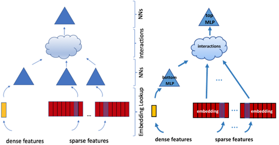
Figure 1. The DLRM model proposed by Facebook AI (left, from [1] without permission) and the actually implemented model (right). Each sparse feature is linearly embedded into a lower-dimensional space. Dense features are processed by the “bottom” MLP. Feature interactions take place in the embedding space shared by the resulting representations of dense and sparse features.
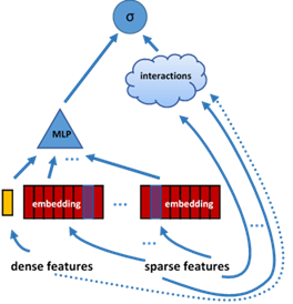
Figure 2. The “Wide and Deep” model [10]. The “deep” component contains a MLP, while the “wide” component deals with cross-products of the sparse features (of a subset of sparse features, to be precise) [10]. In principle, dense features could be factored in into the “wide” component (dotted line).
The source code
We look into the implementation of DLRM as found on the GitHub repository [2] on 16 Nov 2019. The contents of the code repository are listed in Table 1 and include implementations for PyTorch, as well as Caffe2. Everything that is needed to run the model within the PyTorch framework is contained in three files:
- data_utils.py - pre-processes data by parsing text files, forming NumPy arrays and storing them in .npz files (does not use Coffe2 or PyTorch, only NumPy);
- dlrm_data_pytorch.py - implements a custom torch.utils.data.Dataset class which loads data into memory and further transforms it on retrieval; (also contains synthetic dataset implementation, which we do not consider here)
- dlrm_s_pytorch.py - implements DLRM as a custom torch.nn.Module class, as suggested by PyTorch framework.
| Filename(s) | Purpose | |
| /dlrm/ | dlrm_s_caffe2.py; dlrm_s_pytorch.py | model implementation |
| dlrm_data_caffe2.py; dlrm_data_pytorch.py | load data or generate synthetic data | |
| data_utils.py | pre-process dataset files | |
| CODE_OF_CONDUCT.md; CONTRIBUTING.md; README.md | general information | |
| LICENSE | Permissive MIT license | |
| requirements.txt | requires numpy, torch, onnx | |
| kaggle_dac_loss_accuracy_plots.png terabyte_0875_loss_accuracy_plots.png | plots demonstrating convergence in benchmark problems | |
| /dlrm/input | trace.log; dist_emb_*.log | parameters for a synthetic dataset |
| /dlrm/test | dlrm_s_test.sh | script for data-less system health check |
| /dlrm/bench | dlrm_s_benchmark.sh; dlrm_s_criteo_kaggle.sh; dlrm_s_criteo_terabyte.sh | scripts for benchmark tests |
| /dlrm/cython | cython_compile.py; cython_criteo.py | pre-process dataset files faster using cython |
Table 1. The contents of the DLRM GitHub repository [2].
The data and data pre-processing
Although the architecture of DLRM can be applied to various datasets, the paper [1] and the published code [2] work specifically with the datasets published by Criteo Labs [13, 14]. These datasets are online advertisement logs collected over 7 or 24 days and given as text files. Each record in a file corresponds to a shown ad, which may have been clicked by a user, as indicated by a binary label, which is to be predicted by the model. There are 13 integer (dense) features in decimal format and 26 categorical features, each given by an 8-digit hexadecimal hash. Each line contains 40 tab-separated values, some of which may be missing:
The pre-processing is handled by data_utils.getCriteoAdData() function defined in data_utils.py. We do not recommend re-using the code contained in this file for other datasets, as it can be greatly improved. Before using the code with Criteo datasets, we had to make amendments to save categorical features as integers and not floating point values, and to avoid overflow errors when converting a 4-byte positive integer to int32 type. The necessity of these corrections may be caused by a different system setup, package versions, and/or different versions of data files used.
In a nutshell, the data_utils.getCriteoAdData() function parses the input text files, replaces any missing or negative values with zeros, enumerates categorical features according to a dictionary, and saves the result to a .npz file (compressed NumPy format). This file contains arrays of binary target labels, the dense features, the categorical features given by indices, and the array of dictionary sizes for categorical features, which were computed during pre-processing.
Data loading
Data loading in PyTorch is normally done by defining a custom dataset class (subclass of torch.utils.data.Dataset) and passing it to the standard dataloader torch.utils.data.DataLoader, which forms batches of records extracted from the Dataset using a standard or custom collate functions.
The custom dataset class CriteoDataset() is defined in dlrm_data_pytorch.py. Separate dataset objects are initialised for training and test data subsets, as indicated by the parameters passed to the class constructor. If processed .npz files are not found, pre-processing of raw data is initiated as described previously; otherwise, the required subset of data is loaded into memory or buffered. Items are retrieved by dataloader via the CriteoDataset.__getitem__() method, which further transforms the data before returning it on request. This dataset transformation is implemented by CriteoDataset._default_preprocess() method:
- the binary labels are converted to
float32type; - log transformation is applied to the dense features;
- categorical features are cast to
int64type.
After retrieving a necessary number of records from a CriteoDataset() object, a dataloader passes the data to collate_wrapper() function, which is defined in dlrm_data_pytorch.py. This function combines the records into several torch.Tensors, which span the whole batch rather than individual records. Further, the categorical feature arrays are transformed into Compressed Sparse Row (CSR) representation of one-hot encodings, which we will describe in the next section. The torch.Tensors returned by the dataloader are ready to be passed to the model itself.
The model
As shown in Figure 1 (right), the main elements of the DLRM model are (i) the “bottom” MLP, which produces a single embedding for the dense features, (ii) the embedding tables for categorical features, (iii) the “interaction” unit, which provides cross-products of the embeddings and has no learnable parameters, and (iv) the “top” MLP, which does the final processing and yields probabilities.
The key model parameters are passed as command line arguments and specify:
- the dimensionality of the embedding space,
- the number and size of layers in the MLP units,
- whether to compute the “self-interactions” of embeddings.
Following the PyTorch framework, the model is defined as a custom subclass of torch.nn.Module, DLRM_Net. Two obligatory class methods are implemented: the class constructor .__init__() and the .forward() method. The constructor method DLRM_Net.__init__() initialises sub-modules for embeddings and bottom and top MLPs (Figure 1, right), and assigns them to attributes self.emb_l, self.bot_l, self.top_l. Each MLP unit is represented by a torch.nn.Sequential object with torch.nn.Linear, torch.nn.ReLU, and torch.nn.Sigmoid as building blocks. The authors use 5 fully connected layers with ReLU activations in the bottom MLP (of sizes 13, 512, 256, 64, 16) and 3 fully connected layers with ReLU activation followed by a collector node with sigmoid activation function (367, 512, 256, 1) [2]. The embeddings are given by a torch.nn.ModuleList of embedding bags (torch.nn.EmbeddingBag).
Model evaluation (forward pass)
The DLRM_Net.forward() method evaluates the model on a given batch of data. The model can operate in a serial and parallel mode. Here we consider only the serial mode, in which the model evaluation is conducted by DLRM_Net.sequential_forward(), see Figure 3. We introduce the notation for data dimensions in Table 2.
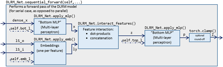
Figure 3. The forward pass of the DLRM model, as implemented by sequential_forward() method using other methods and functions.
| cat - number of categorical features, ln_emb.size |
| dense - number of dense/continuous features, m_den |
| s_p - dictionary size of pth categorical feature, ln_emb[p] |
| emb - the dimension of embeddings of all features, n_emb |
| iter - dimensionality of a dense vector resulting from feature interactions, num_int |
| b - the batch dimension, the number of records processed at once; |
| N_bottom, N_top - number of layers in top and bottom MLPs, including the input layer, ln_bot.size, ln_top.size. |
| n_{l,bottom/top}, l=0,...,N_{bottom/top} - the dimensions of layers in the MLPs, ln_bot[l], ln_top[l]. |
Table 2. Data and model parameters.
The dense features are passed as dense_x, a 2D torch.Tensor, whose major (th) dimension is the batch dimension, and the other (st) dimension refers to various dense features. The dense features are first processed by the bottom MLP, which produces embeddings into the latent space shared by the totality of dense features and individual categorical features. The dimensions of the input and output layers of the bottom MLP must match the number of dense features and the dimensionality of embeddings, respectively,
To describe mathematically what happens to the data, we denote dense_x[i,j]==, where . The bottom MLP is given by
where , and are the th layer’s weights, biases, and activation function. The superscripts are implied but omitted to avoid notation cluttering. The weights and biases are learnt from the data and initialised randomly and independently,
The activation functions are either a rectified linear unit function (ReLU) or a sigmoid function applied element-wise. We can re-write the bottom MLP relation in the batch form,
where the summation over k and the superscripts are implied. The input layer is initialised with , . The output activations are stored into torch.Tensor x, x[i,j]==, see Figure 3.
Now let us look at how the categorical features are processed. The batch values of sparse features are passed in the CSR format, that is, as lists of arrays of indices and offsets. Namely, the batch values of the th feature are given by indices lS_i[p] and offsets lS_o[p], which are torch.Tensors encoding a sparse binary matrix . The CSR format is used by PyTorch module torch.nn.EmbeddingBag, which implements the categorical embeddings in DLRM.
To understand how CSR format works, consider , which is the multi-hot encoding of a single value of p-th categorical feature. This binary row can be unambiguously reconstructed from a list of indices of its non-zero entries. Each row of a sparse binary matrix can be represented this way. The lists of indices for each row are concatenated to form an array of indices, and an array of offsets is supplied to delineate the rows’ boundaries in the concatenation, thereby making it reversible. This pair of integer arrays, lS_i[p] and lS_o[p], is the CSR representation of . In the case of one-hot encoding, which is used for single-valued categorical features in the Criteo Labs datasets, we have simply lS_o[p]==, where , the batch size, equals the number of rows.
Each categorical feature is independently mapped (embedded) into ,
where is the embedding table for the th categorical feature. Embedding tables are learnt parameters and are initialised with independently uniformly distributed random entries,
For a batch input, we have
where the summation over is implied. A list of torch.Tensors is formed to store the embeddings of a batch of inputs, ly[p]==.
The next part of the model is feature interaction. At this stage we have batch embeddings of the vector of dense features and of the categorical features, stored in x and ly, see Figure 3. Let denote these embeddings for a single input. The feature interaction stage computes the scalar products of the embeddings,
and concatenates them together with the dense features embedding . The dimensionality of the resulting vector is
depending on whether “self-interactions” (i.e., squared norms) are included. The computation is done by putting all the embeddings into a single tensor,
multiplying it by its transpose,
then taking the entries below the diagonal, optionally including diagonal elements,
and prepending the embedding of dense features to obtain the result,
For a batch input, we have
where , , . Next, the dot-products are formed
where . Finally, the dense features’ embedding is included to obtain
where , which is stored in torch.Tensor z.
Optionally, the feature interaction module concatenates all the embeddings instead of explicitly computing dot-products.
The output of the feature interaction unit is passed to the top MLP, which is similar to the bottom MLP described previously, but may have different number and dimensionality of layers. The output layer of the top MLP should consist of a single node with sigmoid activation function, which yields batch probabilities
Optionally, DLRM calls torch.clamp() function on the output, which maps each resulting probability to the closest value within some interval , where is some specified threshold. The output of DLRM_Net.sequential_forward() is returned as a 2D torch.Tensor of dimensions -by-1.
Model training
Model training is facilitated by core PyTorch functionality: automatic differentiation (torch.autograd) and automatic optimisation (torch.optim). Automatic differentiation is possible for computations where data is stored by objects of torch.Tensor class or its subclasses and processed by torch.Function’s. Standard arithmetic operators are overloaded in PyTorch, allowing seamless manipulation of torch.Tensors, while a reverse computation graph (“backpropagation graph”) is being constructed in the background. This graph is used to compute gradients of a scalar function (e.g., the loss function) with respect to tensors used in its evaluation directly or indirectly. During the backpropagation each Tensor object accumulates the components of the gradient, corresponding to it, which can later be used for the loss function optimisation.
Automatic optimisation is done using iterative methods, such as stochastic gradient descent. Upon initialisation of an instance of DLRM_Net class, PyTorch modules used in MLP and embedding blocks are set as the instance’s attributes. This causes any tensor parameter of the constituent modules to be registered as parameters of the DLRM_Net module. The optimiser object adjusts these parameters according to the computed gradients and the iterative update rule.
The current implementation of DLRM uses constant learning rate stochastic gradient descent, torch.optim.SGD(), for minimising the loss function given by mean squared error (torch.nn.MSELoss) or binary cross-entropy given torch.nn.BCELoss. The type of loss function and the learning rate can be passed as command line parameters to dlrm_s_pytorch.py call.
Conclusion
We have outlined the state-of-the-art recommendation model DLRM and its implementation, which was open-sourced by the Facebook AI group [1, 2]. This model is in many ways similar to previously proposed models, including “Wide and Deep” [10]. “Deep and Cross” [11], and other models mentioned in [1].
We provided a thorough mathematical description of DLRM and inspected its implementation in PyTorch in more detail than the authors did it. At the same time, we left out the discussion about synthetic datasets, computational bottlenecks, and the performance comparison of DLRM against “Deep and Cross”, for which the reader is referred to the original publication [1].
References
- M. Naumov et al., Deep Learning Recommendation Model for Personalization and Recommendation Systems, (2019) https://arxiv.org/abs/1906.00091
- https://github.com/facebookresearch/dlrm
- M. Naumov and D. Mudigere, DLRM: An advanced, open source deep learning recommendation model, https://ai.facebook.com/blog/dlrm-an-advanced-open-source-deep-learning-recommendation-model/
- K. Lee et al, Big Basin-JBOG Specifications Rev 1.0, (2018) https://www.opencompute.org/documents/facebook-big-basin-jbog-spec
- H.-J. M. Shi et al., Compositional Embeddings Using Complementary Partitions for Memory-Efficient Recommendation Systems, (2019) https://arxiv.org/abs/1909.02107
- A. Ginart et al., Mixed Dimension Embedding with Application to Memory-Efficient Recommendation Systems, (2019), https://arxiv.org/abs/1909.11810
- U. Gupta et al., The Architectural Implications of Facebook’s DNN-based Personalized Recommendation, (2019) https://arxiv.org/abs/1906.03109
- https://github.com/pytorch/glow/blob/master/tests/unittests/RecommendationSystemTest.cpp
- https://github.com/flexflow/FlexFlow/blob/master/examples/DLRM/dlrm.cc
- H.-T. Cheng, Wide & Deep Learning for Recommender Systems, (2016) https://arxiv.org/abs/1606.07792
- R. Wang et al., Deep & Cross Network for Ad Click Predictions, Proceedings of the ADKDD (2017) doi:10.1145/3124749.3124754
- S. Rendle, Factorization Machines, IEEE International Conference on Data Mining (2010) doi:10.1109/ICDM.2010.127
- Criteo Labs Display Advertising Challenge (Kaggle Dataset) https://www.kaggle.com/c/criteo-display-ad-challenge/data
- Criteo Labs Terabyte Click Logs https://labs.criteo.com/2013/12/download-terabyte-click-logs-2/
Large-scale Parallel Collaborative Filtering for the Netflix Prize
Author: Raul Morales DelgadoAuthor: Elham KaramiAuthor: Alireza Darbehani| Author | Contribution |
|---|---|
| Raul Morales Delgado | RMD wrote sections 1, 2, 3.1 and 3.2 |
| Elham Karami | EK wrote sections 3.3 and 4 |
| Alireza Darbehani | wrote sections 5 and 6 |
Large-scale Parallel Collaborative Filtering for the Netflix Prize
Summary
This paper presents a recommendation system technique based on collaborative filtering. Specifically, it proposes and describes the use of the Alternating-Least-Squares with Weighted--Regularization (ALS-WR) parallel algorithm, which was designed for the Netflix Prize. The results achieved with ALS-WR include a model with 1,000 hidden features that obtained a RMSE score of 0.8950 — top of the class for a pure method — and yielded a total improvement of 5.91% over Netflix’s CineMatch recommendation system.
Introduction
The collaborative filtering approach for recommendation systems is based on using the aggregated behavior or taste of a large number of users over a large set of relevant items. In this sense, the main objective of the system is to predict the rating that user will give to an item , which translates into minimizing the root mean squared error (RMSE) between the predicted value and its target.
However, an algorithm that tries to optimize a loss function over a matrix that includes all users and their respective interaction with all items turns out to be computationally expensive — the Netflix Prize proposes a matrix with 100 million ratings (~480,000 users and ~18,000 movies). Given the sparsity of the matrix that was proposed by Netflix, the authors identified a number of problems:
-
The size of the matrix — by the time this paper was presented — was 100 times larger than any previous benchmark datasets.
-
Only 1% of the matrix contained observations, the rest of them were missing.
-
Noise existed in both training and test sets, due to the difficulty of predicting human behavior.
-
The distributions between sets were different — the training set contains data from 1995–2005, while the test set contains only data from 2006.
Finally, it is important to mention that Netflix’s recommendation system had a RMSE score of 0.9514 on the test set, and the objective of the prize was to reduce this score by 10%.
To solve this problem, Zhou et al. presented and described the ALS-WR parallel algorithm, which they ran on Matlab on a Linux cluster, where they achieved a 5.91% improvement on the RMSE score.
As it will be seen in the following sections, the main purpose of ALS-WR is to deal with ill-posed problems and sparse matrices without the risk of overfitting and with models that have a large number of hidden features.
Problem Formulation and Approach Analysis
This section covers section 2 and subsection 3.1 of the original paper. Variables and indices have been conserved from those used in the paper unless specified.
Problem Formulation
Given a user-movie matrix with number of users and number of movies, the resulting matrix can be denoted by
where represents the rating score of movie by user , whether it exists — as a real number — or not — it is missing. In such a case, the objective of a recommendation system would be to estimate some of the missing ratings in .
In order to predict these estimates, one approach is to work with low-rank matrices — two low-rank matrices that would model both the users and the movies through a set of features, and whose multiplication would yield an approximation of . Let us define the user feature matrix and the movie feature matrix as
where is the dimension of the feature space — the number of hidden features that will be considered for each of the above matrices. In other words, column vectors and represent the hidden features for user and movie , respectively, and are a subset of .
Assuming that the ratings are fully predictable and that is sufficiently large, then can be expected. One way to obtain and is by minimizing a loss function, . In the paper, the mean-square loss function is used for that task. For a single rating:
From this expression, an empirical total loss function can be defined as the summation of loss for all ratings:
where is the size of , and is the index set of known ratings.
Therefore, the minimization problem can be formulated as:
By formulating the problem like this, there will be only free parameters to solve for — the index set contains far less user-movie ratings than elements. According to the paper, the dataset provided by Netflix only had 1.1% of known ratings.
The next problem that arises is related to working with such sparse matrix. Specifically, when solving for a relatively large , the resulting feature matrices will overfit the data. To avoid overfitting, a Tikhonov regularization term is appended to :
where and are suitable Tikhonov matrices, which will be discussed in the next subsection.
ALS with Weighted-Regularization Approach
As stated in the paper, a common approach for matrix factorization is using Singular Value Decomposition, SVD, where an approximation to the original matrix is achieved by finding two rank- matrices such that . SVD provides a solution that minimizes the Frobenius norm of .
However, regularized least squares (RLS) methods are preferred when a problem is ill-posed — the number of variables surpasses the number of observations in the dataset — or when, even if the number of observations is larger than the number of variables, the resulting learned model overfits to the dataset. According to Zhou et al., both problems occurred when SVD was applied to the Netflix dataset, so the authors proposed the use of Tikhonov regularization — also known as Ridge regression — to overcome them. Furthermore, they indicate that the inherent sparsity of the user-movie matrix makes it not possible for standard SVD algorithms to find and .
To solve the low-rank matrix factorization problem, the paper proposes the use of alternating least squares (ALS) in the following way:
-
Initializing matrix by assigning the average rating of each movie as the first row and small random numbers for the remaining ones.
-
Holding constant and minimizing for — the sum of squared errors, .
-
Following the completion of the second step, holding constant and minimizing for .
-
Repeating steps 2 and 3 until a stop criterion is satisfied — which, for the proposed model, is a difference of 0.0001 (1 bps) between the observed RMSEs on the probe dataset.
As stated in the previous subsection, the authors deemed necessary the use of Tikhonov regularization, which penalizes large parameters, given that ALS on its own would overfit to the dataset. The Tikhonov matrices they chose for the loss function are stated in the following expression:
where and denote the number of ratings provided by user and the number of ratings that movie has, respectively. Similarly, and are the cardinalities of and , respectively, where represents the set of movies that user rated, and represent the set of users that rated movie . Finally, the authors define the Tikhonov matrices as and — such that —, which will penalize the loss function depending on the number of ratings that each user or movie have.
After is initialized as stated above, in step 1, the following step is to solve for holding constant. will be solved per user — column by column. In other words, will be determined using the regularized least squares loss function provided above, and it will involve the existing ratings by user , and all the hidden feature movie column vectors, , that user has rated. The derivation process is shown in the following lines.
Considering the ALS problem, minimizing the loss function can be achieved as follows:
Given the column vectors,
a partial derivation over will eliminate all variables that do not contain it, and will modify the index set such that now it only contains the set of movies rated by user , . Therefore,
And rearranging the last expression above,
Finally, doing the summations for all ,
And factorizing from the left side of the previous expression:
Where is a sub-matrix of , , is an identity matrix such that , and is the row vector of with columns . If the terms are grouped such that,
then the previous expression can be simplified to:
After this step (step 2) is completed, step 3 can be executed by holding constant and solving for . Using the same procedure as above will yield:
where and . Analogously, is a sub-matrix of , , and is the column vector of with rows .
As shown in this subsection, each iteration of this algorithm will minimize the loss function , which will consequently improve the estimates of the hidden features of and , thus improving the model’s approximation to .
Parallel ALS with Weighted-λ-Regularization
The parallelization of the alternating least square solution (ALS) has been implemented using the MATLAB software package. The latest version of the software allows for several separate MATLAB workspaces, which are running on different hardware platforms, to communicate with each other. Each copy of the software is called a “lab”. The matrices used in the labs can be of three different types:
- Private: each lab has its own copy, and their values differ.
- Replicated: private, but with the same value on all labs.
- Distributed: there is one matrix, but with rows, or columns, partitioned among the labs.
In this step, two distributed versions of the rating matrix R are used. One of them is distributed by rows (i.e., users) and the other by columns (i.e., by movies). To update M (U), the columns (Rows) of R are divided into equal-size blocks and a replicated version of U (M) is used for updating each block. The MATLAB code snippet used for updating one block of M is brought in the paper.
Since the proposed parallelization method uses a distributed algorithm, the only computation cost is the broadcast step, and it takes less than 5% of the total run time.
Performance for the Netflix Prize Problem
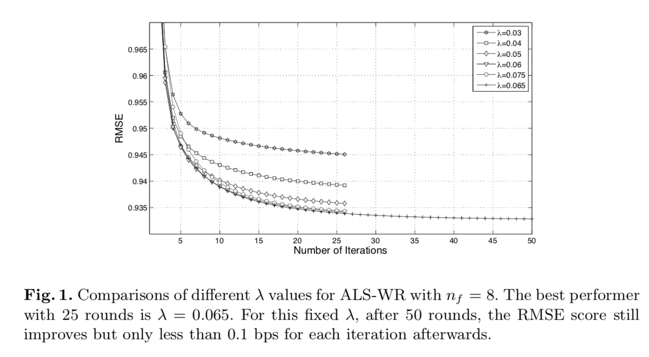
While the test dataset is hidden by Netflix, the training dataset consists of a probe dataset which has the same distribution as the test dataset. As such, the probe dataset is used to optimize the model parameters. The optimal value of lambda is obtained by trial and error, and the iterations for improving the RMSE are stopped when the improvement is less than 1 bps.
Post-processing
The authors propose two post-processing methods for improving the algorithms performance.
- If the mean of the predictions § is not equal to the mean of the test set, it can be corrected by shifting the mean by a constant which equals to: mean(test) - mean§
- Various predictors can be combined linearly to obtain a better predictor.
The details are explained in the paper.
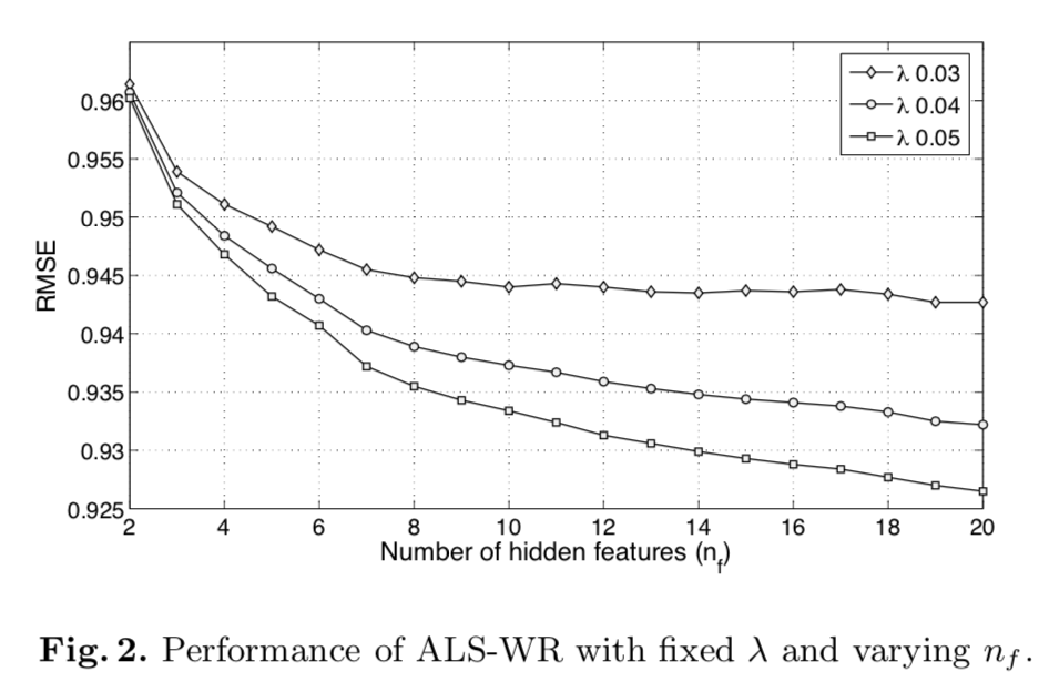
Experimental Results for ALS
The experimental results for finding the optimal values of λ and nf (number of hidden features) are shown in figures 1 and 2, respectively. Figure 1 depicts that with fixed values of λ and nf, the convergence happens after about 20 iterations where the best performer is λ = 0.065. Figure 2 shows that with fixed λ, the RMSE monotonically decreases with larger nf, even though the improvement diminishes gradually. The main finding of these experiments is that the proposed algorithm never overfits the data if the number of iterations or the number of hidden features are increased. A series of experiments with large values of nf indicates that with nf = 1000 an RMSE score of 0.8985 can be obtained which translates into a 5.56% improvement over Netflix’s CineMatch, and it represents one of the top single-method performances.
Other Methods and Linear Blending
Two of the popular collaborative filtering methods include the Restricted Boltzmann Machine (RBM) and the k-nearest neighbor (kNN) method which are implemented and their performances are reported. The RBM is an NN-based method where there are visible states and hidden states, and undirected edges connecting each visible state to each hidden state. To improve performance, both methods are parallelized using MATLAB. For RBM itself, a score of 0.9181 is obtained. For kNN with k = 21 and a good similarity function, a RMSE of 0.9270 is obtained. Linear blending of ALS with kNN and RBM yields a RMSE of 0.8952 (ALS + kNN + RBM), and it represents a 5.91% improvement over Netflix’s CineMatch system.
Related Work
There are similar researches on recommender systems and low-rank matrix approximations and the Netflix Prize in both academia and industry. Here we review a couple of similar researches on each topic:
Recommendation Systems
The recommender Systems research and products are divided into two categories at a high-level view: Content-Based, and Collaborative-Filtering. Collaborative Filtering methods use the behavior of a large set of users against a set of products or choices. In this method, the goal is to make an estimation of what item/product would be the next choice of a user based on the similarity of the user’s previous choices and other users’ choices. Some similar research using Collaborative filtering are GroupLens and Bellcore Video Recommender**. There are also some examples of combining both CF and CB recommenders such as Fab System and Unified Probabilistic Framework. **
Netflix Prize Approaches
The paper Restricted Boltzmann Machines for Collaborative Filtering used the Restricted Boltzmann Machine to obtain a Root Mean Square error score of 0.91 for the Netflix Prize. They also used a Low-Rank Approximation approach which achieved a score of above 0.91 using 20-60 hidden features. They used an SVD function which does the same task as ALS-WR in this paper. However, this paper used 1000 features to improve the score of RMSE.
Another paper (The BellKor Solution to the Netflix Grand Prize) uses a neighborhood based technique that combines the k-nearest neighbor and low-rank approximation. They won the prize in 2007 with the RMSE score of 0.87.
Low-Rank Approximation** **
There are other matrix approximation methods proposed for the Netflix Prize Competition. The paper Collaborative Filtering via Ensembles of Matrix Factorizations proposed nonnegative matrix factorization and maximum margin matrix factorization as the Low-Rank Approximation methods for the Netflix Prize.
Concluding Remarks
This paper introduced a new method to use Collaborative Filtering on large scale data-sets such as the Netflix competition. Slightly better results could be achieved by tweaking the RBM and KNN implementation, however, the goal of this paper was to achieve a significant improvement on the run-time performance by providing parallelization.
Amazon’s item-to-item collaborative filtering
Author: Gurinder Ghotra| Author | Contribution |
|---|---|
| Gurinder Ghotra | GG has solely contributed to this section |
Amazon’s item-to-item collaborative filtering
Some challenges facing Amazon recommendation algorithms
The authors of the paper worked on the many challenges of working with big data for recommendation. For example, due to the huge amount of data, with tens of millions of customers and millions of distinct catalog items, scaling becomes a difficulty. Many applications need results to come in real-time with maximum time lag at half a second, which often isn’t an easy task. Additionally, while there is a lot of data about existing customers, new customers would have extremely limited information making it a challenge to have meaningful recommendations for them. The polar opposite of this could be that older customers can have a glut of information based on their extensive purchase history. The algorithm also needs to be sensitive to changes as Customer data is volatile. Each interaction provides valuable customer data and the algorithm must respond immediately to new info.
Metrics
Metrics that they watch out for and every other email marketing and web based advertisement - the click through and conversion rates.
On these measures item-to-item CF has been very effective.
Other models the author considered
The authors cite 3 common approaches to solving the recommendation problem:
- Traditional collaborative filtering
- Cluster models
- Search-based methods
Most recommendation algorithms fall under 2 categories
-
Based on customers:
- The algorithm starts by finding similar customers based on items searched and ratings given
- The algorithm then aggregates items from similar customers
- Removes the items that a specific user has used and recommends the others
-
Based on items: Herein are search-based and item-to-item collaborative filtering. These algorithms look for similarity in items as opposed to customers. The recommendation is based on proximity of items.
Traditional Collaborative Filtering issues
How it works: The algorithm represents a customer as an N-dimensional vector, where N is the distinct number of items in the catalogue. The components of the vector are positive for purchased or positively rated items and negative for negatively rated items. Best selling items could dominate this vector based on their popularity and positive ratings. The algorithm compensates for best selling items by multiplying the N-dimensional vector with the inverse-frequency (the inverse of the number of customers who have purchased or positively rated the item). This leads to discovery of less well-known items.
The algorithm then makes recommendations based on a few customers that are most similar to the customer. Distance measures like cosine similarity are used.
There are other methods to select items in this algorithm. For instance, for similar customers - ranking of items is based on the number of users purchasing or positively rating the item. Recommendation is based on the top most items.
Limitations of traditional collaborative filtering
Generating recommendations based on collaborative filtering is computationally expensive. With M as number of customers and N as the number of items, the worst case is O(MN).However, since the average customer vector is extremely sparse, the algorithm’s performance is closer to O(M+N). Even with this reduced figure it is quite problematic, as the customer base is over 10 million and the number of items are over 1 million. This leads to severe performance issues when scaling.
Scaling Issues
Since performance is, in practice, O(M+N), one approach is to reduce M, the number of customers. Herein a random sample is taken and this reduced set of customers are used to generate the similarity. As a consequence of using a subset of users, the customers chosen would be less similar to the user as the pool of selection has been reduced.
The other way to tackle scaling is to reduce the number of items, N. Herein the extremes – very popular or highly unpopular items - are disregarded. These items will never be recommended, with another fallout being that customers who have only purchased these extreme range products will not receive any recommendation.
Another approach based on reducing the number of items, N, is to limit the items to a specific product category. The impact is that recommendations would not be able to come from different categories which are not desirable.
Cluster Models
This approach is to convert the recommendation problem to a classification problem. The idea is to identify meaningful clusters based on user information, and then the recommendation for a specific user is based on the cluster the user belongs to. Thus user clusters are generated offline, and then based on online experience, recommendations are provided based on the user cluster. On large data sets optimal clustering is very computationally expensive, hence the data is based on greedy cluster generation. Herein, certain clusters are randomly selected and then each user based on the distance measure such as Euclidean distance is classified into one of these groups. There are provisions for the clusters to be merged. So users are based on similarity to vectors that summarize a segment. These algorithms scale better than traditional collaborative filtering as the computationally expensive portion is done offline and there is a fixed number of clusters to compare against.
The major drawback of cluster based models is that the recommendation quality is low, as effectively everyone in a specific cluster will get the same recommendation, hence personalization is hampered. The solution for this is to build more and more fine-grained clusters. However, if the clusters have few members (in order to achieve better similarity between the members) the number of clusters will increase, and the cluster model suffers from the same issue of scaling and processing time as faced by traditional collaborative filtering.
Search-Based Methods
The third option that the authors of the paper considered was the search-based methods where the recommendation problem is treated as a search for related items. Based on the user’s purchased or positively reviewed items history, the algorithm searches for similar titles, key words, and genre. For example the purchase of the movie the Godfather could trigger a related search for crime drama titles, or other movies directed by the same director, or other movies of the actors.
The algorithm works when the user has few purchases / ratings and can also scale well under this situation. However, when the user has thousands of data points then the search becomes difficult as there are so many query points – numerous key words, genres etc… The solution to this problem is to query based on a subset of the searchable data points. This has a concomitant disadvantage of reducing the recommendation quality.
Item-to-item collaborative filtering
The authors, after considering the three other approaches, honed on to item-to-item collaborative filtering for some key advantages – high recommendation quality even with sparse data, and sub-second recommendation time.
The fundamental idea driving item-to-item collaborative filtering is that users themselves could change their behavior over time, however, the relationship between items tend to stay the same and stand the test of time. This makes for higher recommendation quality.
Item-to-item collaborative filtering matches each of the users’ purchased and rated items to similar items and creates a similarity table. For online recommendation, the algorithm finds similar items to only the items that the user has used or rated, thus substantially reducing the search. It aggregates the similar items, and recommends the most popular or correlated items. The similarity table is generated offline, and the online component is only dependent on the number of items the user has purchased or rated, thus this method allows scaling to even millions of users / items, without an impact to the recommendation time. Moreover, the recommendation is based on similar items, which offers personalized recommendations and maintains high quality.
The authors recommended a pseudo code to generate the item-to-item similarity:
- For each item in product catalog, I1
- For each customer C who purchased I1
- For each item I2 purchased by customer C
- Record that a customer purchased I1 and I2
- For each item I2
- Compute the similarity between I1 and I2 (this could be done by using a distance measure such as cosine similarity)
This code is very computationally expensive with worst case as O(N2M) best cases at O(NM), where N is the number of items and M is the number of customers. However, this computation can be done offline.
Conclusion
The authors tackled the unique problems and requirements that recommendation systems posted in a big data environment - sub-second recommendation and ability to scale to millions of items. They focused on three competing approaches - Traditional collaborative filtering, Cluster methods, and Search-based methods. With each of these methods, the authors found them lacking in the key metrics of scaling and speed of recommendation generation. Item-to-item collaborative filtering was the answer the authors were looking for. The algorithm not only meets the criteria but also works for new customers who have only little data/purchase history.
Pre-training of Context-aware Item Representation for Next Basket Recommendation
Author: Marnie Landon| Author | Contribution |
|---|---|
| Marnie Landon | ML has solely contributed to this section |
Pre-training of Context-aware Item Representation for Next Basket Recommendation
Background
Recommender systems are used by businesses to determine which products their customers are likely to purchase and to keep their customers engaged, and to understand the needs of a given population. In order to personalize the experience for their customers, the system finds patterns in each customer’s purchasing history, and compares each customer to others with similar behaviour or tastes. The patterns are captured in a mathematical model which will predict items that each user is most likely to engage with or purchase.
Market basket analysis is a technique used to discover and model relationships between items that people commonly purchase together, in order to make predictions and find patterns of co-occurrence. The items that a customer buys in a single purchase, transaction, or basket, make up the itemset. The goal is to predict the top K items to recommend for a given user based on a personalized, ranked list. Other names for this method include association analysis or frequent itemset mining. The technique is used for: marketing, physical store layout and website layout, fraud detection, and cross-selling.1 It quickly becomes a combinatorics nightmare, if the inventory is large.
Next basket recommendation is an important part of market basket analysis which aims to recommend a set of items to a user.
The innovation in the paper Pre-training of Context-aware Item Representation for Next Basket Recommendation is to encode the transaction context that captures the purchaser’s intent into an item representation, as opposed to a fixed-length static vector for the item represented by utilizing an embedding layer. The idea had its genesis in the context-aware model used in Natural Language Processing (NLP) called BERT (Bidirectional Encoder Representations from Transformers). The authors replace the word Bidirectional with Item, naming their model IERT. Like BERT, it is a transfer learning approach, using a pre-training phase and a fine-tuning phase. The authors claim to outperform state-of-the-art based on the Ta-Feng data set.
Existing methods
Collaborative filtering (CF)
The goal of Collaborative filtering is to identify users with similar interests and taste and determine what items they liked, and find items similar to items purchased in the past. In other words, by using the behaviour of one customer, it is possible to predict what a similar customer will purchase. The assumption of collaborative filtering models is that similarity determines what a user is most likely to purchase.
Memory based collaborative filtering
Using cosine similarity, find similar users, or pearson correlation and take the weighted average of ratings. There is no training or optimization involved in memory based collaborative filtering.2
Model based collaborative filtering
Machine Learning is used to model user ratings of unrated items. Common methods: 1. Clustering algorithms like KNN; 2. Matrix Factorization like ALS; 3. Deep Neural Networks. 2
Deep Neural Network (DNN) approaches:
HRM - Hierarchical Representation Model captures how the purchase of one item relates to the purchase of another item, sequential behaviours, the purchaser’s interests, and general taste.
DREAM – Dynamic REcurrent bAsket Model builds on HRM, using RNNs to model the sequential relationships of itemsets.
ANAM- Attribute-Aware Neural Attention Model – also uses the attention architecture to adapt to a purchaser’s changing interests.
All of the deep learning approaches used prior to this paper model user-item interactions and item-item interactions, using a fixed-length static vector representation of the items. As mentioned in the introduction, the proposal in this paper is to represent the user’s intentions with the item representation in a context-aware style, similar to BERT.
BERT
On October 11, 2018, a team from Google AI Language published a seminal paper that transformed (pun intended) Natural Language Processing (NLP). Previously, bi-directional Long Short-Term Memory (BiLSTM) models, a specific implementation of the Recurrent Neural Network (RNN) architecture, were used to capture left-to-right and right-to-left context aware representations of words that were concatenated in a “shallow” way. BERT was the first model to use deep bi-directional context-aware representation of words, disambiguating words, increasing the semantic representation captured from the surrounding text, without the use of RNNs. RNNs had significant limitations in capturing long term dependencies between words.
The inspiration for BERT came from a language comprehension and vocabulary test proposed by W. L Taylor in 1953, the Cloze task. The goal of the Cloze task is to fill in missing words from a passage of text.
There are two tasks in the pre-training phase of BERT:
-
Masked Language Model (MLM)
15% of all WordPiece tokens in each sequence are randomly “masked” or hidden. The model is trained using cross entropy loss to predict the original token.
-
Next Sentence Prediction (NSP)
A model is trained to predict the relationship between sentences from labelled sentence pairs. 50% of the time the label is IsNext, the other 50% are labelled NotNext.
Following the pre-training phase, BERT uses a fine-tuning approach or feature-based approach. The fine-tuning phase adds a simple classification layer to the pre-trained model. The feature-based approach extracts fixed features from the pre-trained model and runs computationally inexpensive models using these representations.
Fundamentally, once you understand BERT, you can think of IERT as using the concept of a word in BERT as an item; and a sentence as a basket; and a document as a sequence of baskets. The similarities and differences of BERT and IERT are in the table below.
| BERT | IERT |
| Similarities | |
| word | item |
| sentence | basket |
| document | sequence of baskets |
| MLM Masked Language Model | Masked Item Prediction |
| NSP Next Sentence Prediction | Next Basket Prediction |
| Differences | |
| word and sentence order embedded | order information among transactions embedded, item order within a transaction NOT embedded* |
| Sentence pair relationship representation | intention-related transaction representations |
| Same word in different datasets has a similar meaning | Item ID not consistent across datasets** |
* Order embedding: if you scramble the order of the words in a sentence, or the order of sentences in a document, it makes it difficult, maybe impossible, to understand. However, with items in a shopping basket, the order does not give you any additional information about the users’ interests, tastes, or intention. It doesn’t matter if you buy milk and then vegetables, or vegetables and then milk. Therefore, within a given transaction, the order is not embedded. To capture any temporal patterns, order information among transactions is embedded. If you buy milk every four weeks, it is useful predictive information to capture.
** Using the Attention mechanism, both local and global behaviours are captured. Local features are from the current interaction. Global features are item-item or user-item over all interactions.
Conclusion
Modelling user intent is a fundamental objective of recommender systems. Combining frequency-based recommender systems, which use a user’s page visiting history, and content-based recommendation systems, which use various techniques to measure the relevance of content to a user, the authors of the paper Intent-Aware Contextual Recommendation System5 attempt to model what the user wants to do and needs to do.
In this paper, Pre-training of Context-aware Item Representation for Next Basket Recommendation, the authors argue that an item purchased for one purpose should be encoded differently than the same item used for a different purpose. The NLP model BERT inspired, context-aware item representation in a next basket recommendation model is called IERT. The pre-training uses historical purchase transactions. The fine-tuning is done during the online recommendation. However, unlike words in a text document, which have context and inherent structure within a document, items in a basket lack a coherent structure, and there can be a myriad of motivations for an item purchase that change over time for any given user.
If I purchase several baby items, I could be having a shower for my neighbour, or about to become a parent, or saw a discount on baby items and want to stash baby shower gifts on bulk; the list of possibilities goes on. Maybe while I am buying my baby items, I see an advertisement for something that grabs my attention and I add that to my shopping basket, along with the regular items I order like paper towels and dish soap. Is the crib in scenario one different semantically than the crib in the other scenarios from the perspective of predictive power? Do the items in my basket that are not part of my baby shopping add any relevant context to the crib that should be embedded in the item representation?
In other words, a basket does not tell a story like a written document does, and the disambiguation problem in natural language understanding is a different cognitive process than speculating on the possible intent, or motivation(s), of a purchase. BERT is modelled after human reading comprehension strategies, which require the words surrounding the target word to provide context, in order to embed the appropriate semantic representation of the word. IERT, on the other hand, maps the idea of sentence onto a basket of items, and the idea of document onto a sequence of baskets, which, I would argue, are conceptually different. A crib purchase can indicate a baby in the life of the shopper, but the various intentions for the purchase of that crib can not be determined from the shopping history, and the traditional lookup for crib seems to be an efficient method to gain the necessary prediction information.
Furthermore, Amazon, as an example, sells more than 353 million products.3 The English language has approximately 170,000 words.4 Given the possible combinations of items in a basket, and the myriad of possible intentions for each item at any given time, it seems very ambitious for a very large inventory with diverse user populations to achieve realistic results, as claimed. I remain sceptical that intent can be modelled for every item in a shopping basket using natural language processing techniques similar to BERT!
-
https://www.statisticshowto.datasciencecentral.com/market-basket-analysis/
-
https://towardsdatascience.com/various-implementations-of-collaborative-filtering-100385c6dfe0
-
https://www.retailtouchpoints.com/resources/type/infographics/how-many-products-does-amazon-carry
-
https://wordcounter.io/blog/how-many-words-are-in-the-english-language/
-
https://arxiv.org/pdf/1711.10558.pdf Intent-Aware Contextual Recommendation System 28 Nov 2017