Generative Adversarial Networks; an Overview
Contributors: Ali DarbehaniAlice RuedaAmir Namavar JahromiDoug RangelGurinder GhotraMost Husne JahanParivash AshrafiRobert HensleyTryambak KaushikWilly RempelYony Bresler
This blog post is the collective work of the participants of the “GAN” workshop organized by Aggregate Intellect. This post serves as a proof of work, and covers some of the concepts covered in the workshop in addition to advanced concepts pursued by the participants.
Table of Contents
- Introduction
- Semi-supervised learning with Generative Adversarial Networks
- Large Scale Adversarial Representation Learning
- Semi-supervised Learning with GANs: Manifold Invariance with Improved Inference
- Progressive Growing Of GANs For Improved Quality, Stability, And Variation
- Evolutionary Generative Adversarial Networks
Introduction
Author: Willy Rempel| Author | Contribution |
|---|---|
| Willy Rempel |
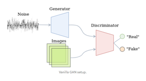
A generative adversarial network (GAN) is a class of machine learning systems where two neural networks, a generator and a discriminator, contest against each other. The goal is for the system to learn to generate new data with the same statistics as the training set. The most common dataset used is a dataset with images of flowers.
The input of the generator is a random vector drawn from some chosen probability distribution. This is referred to as the latent space. The output is of the same dimension as the real data that the generator is attempting to mimic. This – as well as batches of real data for training – is then fed as input into what is called the discriminator. The discriminator attempts to discriminate between the real and generated input. Its sole output is binary: ‘fake’ or ‘real’.
There are 2 popular GAN architectures to note.
First, deep convolutional GANs (DCGANs). These are a category of models in which convolutional layers are used to learn features through which the input distribution is turned into the target distribution.
They are defined by specific architectural decisions:
-
Pooling layers are removed, and only convolutions are used.
-
For the generator, inverse convolutions progressively increase the dimensionality of the tensors to finally match that of the intended output image. Usually the number of channels are correspondingly reduced.
-
The discriminator uses strided convolutions with arguments chosen such that we end with the final layer of a single binary decision node ‘yes/no’.
-
Batch normalization is used for each layer.
-
LeakyReLUs are the sole activation function, except for the final layers of the networks:
-
The generator’s final layer uses
tanhas the activation function. -
The discriminator’s final activation function is a sigmoid.
The second GAN architecture of interest is the cycleGAN. To train cycleGAN, two datasets are used, coming from different distributions. The most commonly used datasets for cycleGANs are sets of images. For example, one set could be winter landscape scenes and the other set summer scenes. The cycleGAN attempts to learn what is unique from each dataset, such that the generators could take any image from the one set and convert it into the ‘style’ of the other set. In other words, the image is taken from one distribution and transformed such that the discriminator would recognize it as a member of the other distribution.
Two GANs are used in this case. For datasets and , we have:
, where is interpreted as 's approximation of
, similar to above
Notice that in this case the generators no longer take random vectors as input, but images instead.
The discriminators , are trained, similar to the above equations, to discriminate between real images from the datasets and fake images from the generators. However, for the generators we train not just to fool the discriminator, but for cycle consistency:
For we have, .
Likewise for , we have
The loss functions are defined in terms of the difference between the original image and its corresponding recreation via both generators. This cycle loss is added to the usual loss during training.
The primary motivation for cycle consistency is that image pairing between the two training datasets is not required. That is, the generator does not need to target a particular corresponding image for a given input. Image pairing would require a correct image in the target domain for every input image. For the example of style transfer, the target image would need to be exactly like the input image, save for the addition of the style of the target domain. This greatly reduces the availability of data and would likely involve manual curation.
The structure of this article is as follows:
Firstly, the original GAN (Goodfellow 2014) is introduced, and the application of GANs for multi-label classification (Odena 2016) is discussed in detail. Various GAN structures such as BiGAN, BigGAN, and BigBiGAN are then explained. A variation of BiGAN, which modifies the discriminator’s loss function, is discussed, as well as other types of variations such as Progressive Growth of GANs (by incrementing the resolution of image pixels) and evolutionary methods (with code reproduction and tutorial), are then respectively explained in detail.
Semi-supervised learning with Generative Adversarial Networks
Author: Tryambak Kaushik| Author | Contribution |
|---|---|
| Tryambak Kaushik | TK has solely contributed to this section |
The original GAN (Goodfellow, 2014) (https://arxiv.org/abs/1406.2661) is a generative model, where a neural-network is trained to generate realistic images from random noisy input data. GANs generate predicted data by exploiting a competition between two neural networks, a generator () and a discriminator (), where both networks are engaged in prediction tasks. generates “fake” images from the input data, and compares the predicted data (output from ) to the real data with results fed back to . The cyclical loop between and is repeated several times to minimize the difference between predicted and ground truth data sets and improve the performance of , i.e., is used to improve the performance of .
The paper discussed in this post, Semi-supervised learning with Generative Adversarial Networks (https://arxiv.org/abs/1606.01583), utilizes a GAN architecture for multi-label classification.
In order to demonstrate a proof of concept, the authors (Odena, 2016) use the MNIST image dataset. MNIST is a popular multi-label classification dataset and is extensively used to evaluate the performance of supervised learning algorithms in classifying dataset images into classes. Note that the authors used image datasets, but the concepts can be easily implemented for other datasets as well.
In the current GAN implementation, classifies images into one of classes, where is the number of pre-defined classes and is the additional class to predict the class of output from . In other words, performs “supervised” classification of a given image with possible classes (or labels) and an “un-supervised” classification with class to determine if the image is real or fake. on the other hand generates increasingly realistic fake images which are fed to , which forces to improve its performance in determining if an image is real or fake, as well as classifying it into one of the MNIST labels. Thus, is used to improve the performance of in the current paper, which is a role that is reversed compared to original GAN paper. This implementation is defined as Semi-supervised Generative Adversarial Networks (SGAN).
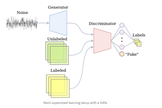
Notes: Images from https://medium.com/@jos.vandewolfshaar/semi-supervised-learning-with-gans-23255865d0a4
The authors achieve this by replacing the sigmoid function in with a softmax function.
The model is shown to improve classification performance, especially for small datasets, by up to 5 basis points above classification using simple convolution neural networks (CNNs) .
SGAN is also shown by the author to generate better predicted images than a regular GAN.
The discussion of SGAN henceforth is divided into the following sections:
-
Uploading and visualizing the data
-
Defining and
-
The training loop
-
Results
1. Uploading and visualizing the data
Pytorch libraries offer the MNIST data set and it can be easily loaded for the current analysis as follows:
train_set = dset.MNIST(root='./data', train=True, transform=trans)
The use of dset allows us to transform the raw dataset to resize, crop, change to the tensor data type, and normalize.
trans = transforms.Compose([transforms.Resize(image_size),

transforms.CenterCrop(image_size),

transforms.ToTensor(),

transforms.Normalize([0.5], [0.5])])
The MNIST training dataset has 6000 pairs of images and labels. Training the model on all these pairs simultaneously would require extensive computational resources. Therefore, the dataset is divided into many batches of a pre-defined small number of dataset pairs. This implementation requires less computational resources to train as the model trains only one batch at a time. Pytorch’s DataLoader offers a convenient way to create batches for training.
train_loader = torch.utils.data.DataLoader(

dataset=train_set,

batch_size=batch_size,

shuffle=True)
In order to verify its contents, the data-loader is iterated to display a batch of 25 images and labels.
2. Defining and
The Generator () of the adversarial network is used to upscale noisy data to a meaningful image. Upscaling in the current context refers to increasing the tensor dimensions of the noisy data (from X1X1 to 1X28X28, where is length of noise vector). In the current implementation, consists of a linear layer followed by 3 hidden layers. Specifically, the hidden layers consist of 2 convolutional layers of type ConvTranspose2D with batch normalization, and 1 convolution layer without batch normalization. The logits output from the final convolution layer are activated with a tanh function.
The Discriminator () of the adversarial network, on the other hand, is used to downscale the image input to a pre-defined number of classes (or labels) of the classification problem. Opposite to upscaling, downscaling refers to decreasing the tensor dimensions (from 1X28X28 to 10X1X1). This downscaling is achieved with a combination of 3 hidden convolution layers of type Conv2D with batch normalization and 1 hidden linear layer.
The of a semi-supervised GAN has two tasks: 1) Supervised learning and 2) Unsupervised learning. Hence, 2 activation functions, softmax and sigmoid, respectively, are defined within the GAN discriminator. The Softmax outputs 10 logits (for 10 possible output classes) for each image for multi-label classification, while the sigmoid outputs 1 logit to indicate a real or fake classification.
The loss function for supervised learning is also consequently defined as CrossEntropyLoss and BCELoss for supervised learning and semi-supervised learning, respectively.
Adam optimizer of stochastic gradient descent is used to update the weights of the neural network.
3. Training Loop
The training loop consists of two nested loops. The inner loop trains and over all the data batches defined earlier with DataLoader. The outer loop repeats this process on the training dataset 200 times (200 epochs).
The training within each loop is executed separately for supervised and unsupervised learning.
The unsupervised learning implementation is similar to a classical GAN, where the discriminator is trained on both real and fake data. Similar to a vanilla GAN, fake data is the output from the Generator () model, and it is fed as input into model for binary (real/fake) classification.
However, the supervised learning implementation of SGAN is different from classical supervised learning algorithms, as SGAN models trains only on half MNIST training dataset, i.e., SGAN is able to achieve higher prediction accuracy by training only on half of the dataset. In fact, the nomenclature “Semi-supervised” learning derives itself from this modified GAN architecture. Furthermore, this implementation also prevents model overfitting as half of the training data set is not used to train the model.
The weights of and are initialized to a random normal distribution with zero mean and 0.02 standard deviation, before the start of training.
Binary Cross Entropy Loss function is used to calculate loss for and unsupervised , while Cross Entropy Loss function is used to calculate loss for supervised . The total loss, is thus, sum of supervised loss and unsupervised loss.
Adam optimizer is used to update the weights of and . The models are back propagated to implement the gradients and update the training weights at the end of each loop. However, to prevent gradient accumulation after each loop and avoid mix-up between mini-batches, the models are re-initialized as zero_grad() at the start of each loop.
After the model was trained on train dataset, it (the trained model ) was used to predict the image’s MNIST label for the test dataset.
4. Result Visualization
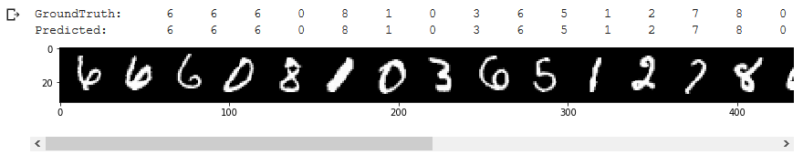
performs extremely well in predicting labels of MNIST ‘test-dataset’, reaching an accuracy of 98%. The result is also very encouraging considering that only half of the training dataset was used to train .

Further validating ‘s performance, predicted values match the groundtruth values of ‘train-dataset’ in the visual data comparison.
Large Scale Adversarial Representation Learning
Author: Most Husne JahanAuthor: Robert HensleyAuthor: Gurinder Ghotra| Author | Contribution |
|---|---|
| Most Husne Jahan | MHJ summarized the comparison among BiGAN, BigGAN, BigBiGAN |
| Robert Hensley | RH provided the section on the “BigBiGAN basic structures compared to the Standard GAN |
| Gurinder Ghotra | GG summarized BigBiGAN |
1. Comparison of BiGAN, BigGAN, and BigBiGAN
BiGAN: Bidirectional Generative Adversarial Networks (BiGANs)
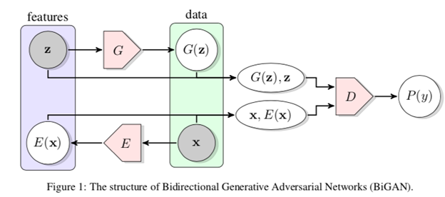
Figure 1: The structure of Bidirectional Generative Adversarial Networks (BiGAN).
GANs can be used for unsupervised learning where a generator maps latent samples to generate data, but this framework does not include an inverse mapping from data to latent representation.
BiGAN adds an encoder to the standard generator-discriminator GAN architecture — the encoder takes input data and outputs a latent representation z of the input. The BiGAN discriminator D discriminates not only in data space ( versus ), but jointly in data and latent space (tuples versus , where the latent component is either an encoder output or a generator input .
BigGAN: LARGE SCALE GAN TRAINING FOR HIGH FIDELITY NATURAL IMAGE SYNTHESIS
BigGAN essentially allows scaling of traditional GAN models. This results in GAN models with more parameters (e.g. more feature maps), larger batch sizes, and architectural changes. The BigGAN architecture also introduces a “truncation trick” used during image generation which results in an improvement in image quality. A specific regularization technique is used to support this trick. For image synthesis use cases, truncation trick involves using a different distribution of samples for the generator’s latent space during training than during inference. This “truncation trick” is a Gaussian distribution during training, but during inference a truncated Gaussian is used - where values above a given threshold are resampled. The resulting approach is capable of generating larger and higher-quality images than traditional GANs, such as 256×256 and 512×512 images. The authors proposed a model (BigGAN) with modifications focused on the following aspects:
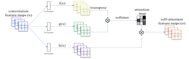
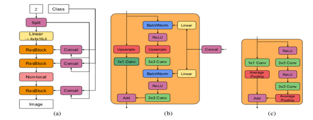
Figure 2: Summary of the Self-Attention Module Used in the Self-Attention GAN
| Contribution | ||
| 1 | Self-Attention Module and Hinge Loss | BigGAN uses the model architecture with attention modules from SAGAN and is trained via hinge loss |
| 2 | Class Conditional Information | The class information is provided to the generator model via class-conditional batch normalization |
| 3 | Spectral Normalization | The weights of the generator are normalized using spectral normalization |
| 4 | Update Discriminator More Than Generator | In the original GAN training algorithm, it is common to first update the discriminator model and then to update the generator model. BigGAN slightly modifies this and updates the discriminator model twice before updating the generator model in each training iteration. |
| 5 | Moving Average of Model Weights | The generator model is evaluated based on the images that are generated |
| 6 | Orthogonal Weight Initialization | Model weights are initialized using Orthogonal Initialization |
| 7 | Larger Batch Size | Very large batch sizes were tested and evaluated |
| 8 | More Model Parameters | The number of model parameters was also dramatically increased |
| 9 | Skip-z Connections | Skip connections were added to the generator model to directly connect the input latent point to specific layers deep in the network |
| 10 | Truncation Trick | The truncation trick involves using a restricted (truncated) distribution for latent space samples. This leads to better resolution at the cost of less sample variety |
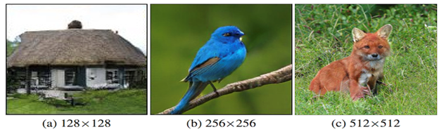
_Figure 3: Sample images generated by BigGAN_s
BigBiGAN – bi-directional BigGAN: Large Scale Adversarial Representation Learning
(Unsupervised Representation Learning)
Researchers introduced BigBiGAN which is built upon the state-of-the-art BigGAN model, extending it to representation learning by adding an encoder and modifying the discriminator. BigBiGAN is a combination of BigGAN and BiGAN which explores the potential of GANs for a wide range of applications, like unsupervised representation learning and unconditional image generation.
It has been shown that BigBiGAN (BiGAN with BigGAN generator) matches the state of the art in unsupervised representation learning on ImageNet. The authors proposed a more stable version of the joint discriminator for BigBiGAN, compared to the discriminator used previously. They also have shown that the representation learning objective also helps unconditional image generation.
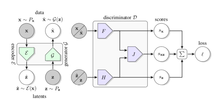
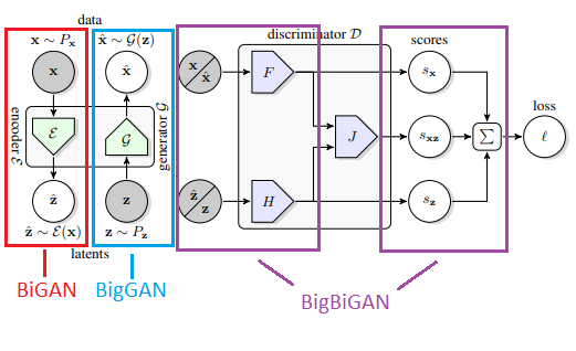
Figure 4: An annotated illustration of the architecture of BigBiGAN. The red section is derived from BiGAN, whereas the blue sections are based on the BigGAN structure with the modified discriminators
The above figure shows the structure of the BigBiGAN framework, where a joint discriminator is used to compute the loss. Its inputs are data-latent representation pairs, either , , sampled from the data distribution and encoder outputs, or , sampled from the generator outputs and the latent distribution . The loss includes the unary data term and the unary latent term , as well as the joint term which ties the data and latent distributions.
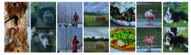
Figure 5: Selected reconstructions from an unsupervised BigBiGAN model
In summary, BigBiGAN represents progress in image generation quality that translates to substantially improved representation learning performance.
Ref:
-
BiGAN Paper: https://arxiv.org/pdf/1605.09782.pdf
-
BigBiGAN Paper: https://arxiv.org/pdf/1907.02544.pdf
-
BigGAN Paper: https://arxiv.org/pdf/1809.11096.pdf
2. Ablation study conducted for BigBiGAN:
As an ablation study, different elements in the BigBiGAN architecture were removed in order to better understand the effects of the respective elements. The metrics used for the study were IS and FID scores. IS score measures convergence to major modes while FID score measures how well the entire distribution is represented. A higher IS score is considered to be better, whereas a lower FID score is considered better. The following points highlight the findings of the ablation study:
- Latent distribution Pz and stochastic E.
The study upholds the findings of BIG-GAN of using random sampling from the latent space as a superior method.
-
Unary loss terms:
-
Removing both the terms is equal to using BI-GAN.
-
Removing leads to inferior results in classification as represents the standard generator loss in the base GAN.
-
Removing does not have much impact on classification accuracy.
-
Keeping only has a negative impact on classification accuracy.
Divergence in the IS and FID score led to the postulation that the BIG-Bi-GAN may be forcing the generator to produce distinguishable outputs across the entire latent space, rather than collapsing large volumes of latent space into a single mode of data distribution.
-
It would have been interesting to see how much improvement the unary terms impose with the reduction of generator from BIG-GAN to DCGAN, this change of generator would have conclusively shown their advantage.
-
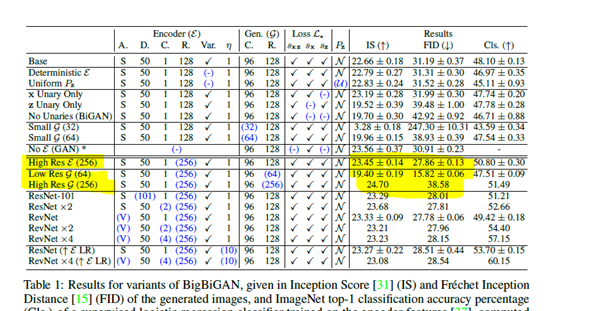
Table of
ISandFIDscores (with relevant scores highlighted):
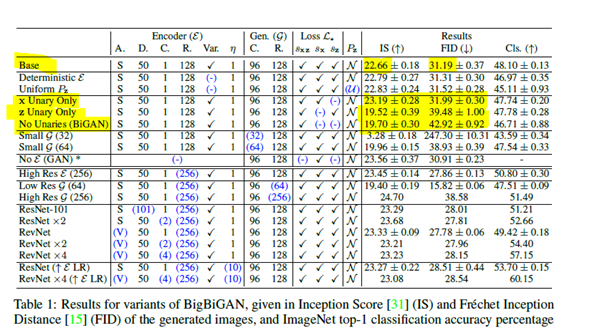
Table 1: Results for variants of BigBiGAN, given in Inception Score (IS) and Fréchet Inception Distance (FID) of the generated images, and ImageNET top-1 classification accuracy percentage
3. Generator Capacity
They found that generator capacity was critical to the results. By reducing the generator’s capacity, the researchers saw a reduction in classification accuracy. The generator was changed from DCGAN to BIG-GAN, which is a key contributor to its success.
4. Comparison to Standard Big-GAN
BigBiGAN without the encoder and with only the unary term was found to produce a worse IS metric and the same FID metric when compared to BIG-GAN. From this, the researchers postulated that the addition of the encoder and the new joint discriminator did not decrease the generated image quality as can be seen from the FID score. The reason for a lower IS score is attributed to reasons similar to the ones for unary term (as in point 2 - Unary loss term).
5. Higher resolution input for Encoder with varying resolution output from Generator
Big-GAN uses
-
Higher resolution for the encoder.
-
Lower resolution for generator and discriminator.
-
They experimented with varying resolution sizes for the encoder and the generator and concluded that an increase in the resolution of the generator with a fixed high resolution for the encoder improves performance.
Note: looking at the table (the relevant portion is highlighted) this seems to be the case only with IS and not with FID, which increases to 38.58 from 15.82 when we go from low resolution for the generator to high resolution.
6. Decoupled Encoder / Generator optimizer:
Changing the learning rate for the encoder dramatically improved training and the final representation. Using a 10X higher learning rate for the encoder while keeping the generator learning rate fixed led to better results.
7. BigBiGAN basic structures compared to the Standard GAN
At the heart of the standard GAN is a generator and a discriminator. The BigBiGAN expands on this, building on the work of BiGAN and BigGAN, to include an encoder and “unary” term discriminators ( and ) which are then jointly discriminated along the lines of “encoder vs generator” through the final discriminator (). As a result of these additions, some natural model changes emerge.
Change in the discrimination paradigm
Where the standard GAN discriminates between ‘real’ and ‘fake’ inputs, the BigBiGAN shifts that paradigm slightly to discriminating between ‘encoder’ and ‘generator’. If you think about the model in terms of “real” and “fake” you might be tempted to think about the real latent space as “real” and the fake latent space as “fake” – this is different than what they do, and is important to the reason why we should notice the shift towards encoder vs generator. From this point on, each discriminator will be seen as discriminating “encoder from generator” and no longer “real from fake.”
Other natural model changes that emerge from the addition of an encoder and unary terms
Since the generator attempts to generate images, and the encoder attempts to generate latent space (aka the “noise” in the standard GAN), the structure of the outputs are different shapes. The image shapes are handled similar to a DCGAN, and the latent space shapes are handled with linear layers like the original GAN. As a result, the discriminator is a CNN that discriminates between encoder and generator images, while the discriminator is a linear module that accepts a flattened input and discriminates between encoder and generator latent space.
After the first phase of discrimination, the outputs of are flattened so they can be concatenated with outputs, then and outputs are jointly fed into the final discriminator . As such, will then discriminate between the concatenated encoder values , and the concatenated generator values which can also be written as .
For scoring , , and - with F_out and H_out needing to be matrices that can be feed into - reducing F_out and H_out to a scalar needs to be done after their respective discrimination. Off the back of this requirement emerges the terms , and . These are linear layers that simply reduce , and each to a scalar that can then be summed up () and scored.
Compared to the standard GAN that is discriminating real values from fake values: () from , the BigBiGAN can be seen as similarly discriminating a group of encoder values from a group of generator values: () from ().
Semi-supervised Learning with GANs: Manifold Invariance with Improved Inference
Author: Parivash AshrafiAuthor: Doug RangelAuthor: Yony Bresler| Author | Contribution |
|---|---|
| Parivash Ashrafi | PA provided Method/conclusions |
| Doug Rangel | DR provided results |
| Yony Bresler | YB provided intro/outline |
Introduction
GANs are normally used for unsupervised learning tasks, where real data is used to train the Discriminator, , as well as the Generator . If the discriminator identified the input as real it outputs , and conversely if it identified as fake. One extension of the traditional GAN structure is to have the discriminator classify real inputs in addition to detecting fake data. The modification to the GAN discriminator is relatively straightforward: for labels that may be classified, denotes that the discriminator identified the input as having label , and if it is identified as fake. This is advantageous as it is possible to train the discriminator classifier even if the number of available labeled data is small compared to unlabeled data.
The success of the semi-supervised GANs relies on the manifold hypothesis, which states that the real classification data lies in a low dimensional manifold within a much larger dimensional space. For example, images with handwriting occupy a much smaller space than the space of all possible pixel images.
In this paper, the authors suggest that, as the GAN is able to well describe the manifold, it can be further used to study the tangent space to that manifold. Rather than manually assuming the invariances of the manifold (e.g. rotational, translational invariance, as done in other methods), this method automatically detects the invariances present in the manifold, leading to improved results over previous semi-supervised classifiers.
Method
This model has three important components, as exists in the BIGAN model, which are an encoder (), a generator (), and a discriminator (). The generator and encoder are trained jointly using the adversarial training where the pair is considered a fake example () and the pair is considered a real example by the discriminator ( is the input noise and is the real data). This model’s first difference from BIGAN is a modification in the discriminator’s loss to optimize the generator and encoder. Feature matching loss is also added to the generator’s loss function, and computed using features from an intermediate layer of the discriminator. This loss minimizes the statistical difference between the features of the real images and the generated images.
To improve the convergence of the model, a third pair, , which is also considered by the discriminator as a fake example, is added to the loss (augmented-BIGAN). Evaluation of the model with regard to similarity between and showed that Augmented-BiGAN works significantly better than BiGAN both quantitatively and qualitatively.
In order to estimate the dominant tangent space,the Jacobian of at , is calculated. Since only the dominant tangent directions in the row span of is needed, the authors use SVD on the matrix and consider the right singular vectors corresponding to top singular values ( is pre-trained). In order to add invariances (such as rotation, translation, etc) to the classifier using tangents, they also add a regularization term (Jacobian of the classifier function ) which penalizes the linearized variations of the classifier output along the tangent directions .
Furthermore, to train the GAN on a semi-supervised manner, the discriminator also serves as a classifier. For a semi-supervised learning problem with k classes, the discriminator has outputs which the th output corresponds to the fake examples obtained from the generator of the GAN. The discriminator’s loss function for this model is the loss of unsupervised training plus the loss of supervised training. The unsupervised loss component is the same as the regular GAN discriminator loss, with the only modification that there are now outputs. As mentioned earlier, for adding invariance to the classifier, in addition to the supervised and unsupervised loss functions, the feature matching GAN with semi-supervised loss is added to the final loss function.
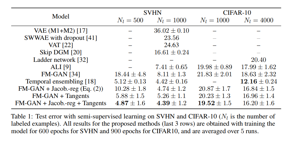
Results
Significant improvements were achieved over baselines, particularly for SVHN and 500 labeled examples, where the test error was reduced from 5.12 (Temporal ensembling) to 4.87 after 600 epochs, averaged over 5 runs. On CIFAR10, improvements were not as good, with the state-of-the-art still belonging to Temporal ensembling. FM-GAN reached similar test error to ALI on 1000 labeled examples, however it managed to do so by using 900 epochs only, while ALI used 6,475. The authors believe that combining the method introduced by FM-GAN with Temporal ensembling could further improve state-of-the-art for semi-supervised learning results.
Conclusion
The results from the paper show that in general, using the tangents of the data manifold that comes from the generator improves the performance of the semi-supervised learning task, as it can add invariance such as rotation and translation into each of the classes, without the need for adding more labeled data. In addition, using fake examples with different difficulty levels to the semi-supervised learning with GANs was effective in the model performance. One suggestion for this can be having a distortion model that takes as input the real examples and distorts them, where the strength could be controllable.
Progressive Growing Of GANs For Improved Quality, Stability, And Variation
Author: Amir Namavar JahromiAuthor: Ali Darbehani| Author | Contribution |
|---|---|
| Amir Namavar Jahromi | ANJ drafted the script |
| Ali Darbehani | AD editted the script |
1. Introduction
The PGGAN (Progressive Growing of GAN) paper is about building a GAN model to generate high-resolution outputs (images in figure 1) progressively. However, the generation of high-resolution images is difficult because higher resolution makes it easier to tell the generated images apart from training images. To generate high-resolution images and also solve this problem, the authors propose a progressive approach that starts with a simple generator and discriminator (low-resolution images) and adds more complex (bigger) layers to both of the models simultaneously to obtain higher resolution images. Figure 1 shows the procedure of PGGAN. This procedure has two advantages compared to other GAN models: 1) the model is more stable than the previous ones, since the small layers that generate large-scale structures are less dependant on class information, and 2) this technique reduces training time since the smaller layers trained more often than, the bigger one and they are easy and fast to train.
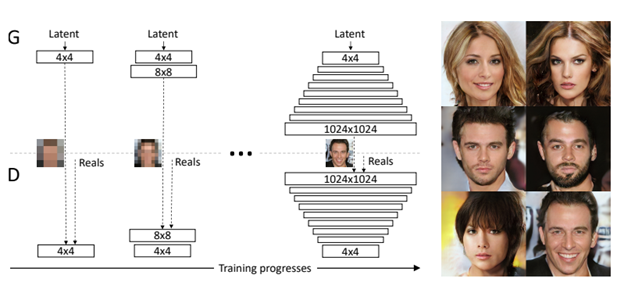
Figure 1. The training starts with both the generator () and discriminator () having a low spatial resolution of 4×4 pixels. New layers are added to and incrementally to increase the spatial resolution of the generated images.
2. Method
The incremental procedure allows the model to learn the large-scale structure of the image distribution (using the simpler networks) and then shift to the finer scale detail (using deeper networks), instead of learning all scales simultaneously.
The generator and discriminator are mirror images of each other and image sizes and number of layers are increased and mirrored. All layers of these two networks are trainable in all training steps. To prevent sudden shocks to the network by adding a new layer, they fade in the layer smoothly (see Figure 2). To do this, they add the weighted result of the up-sampled result of last layer with the result of the new layer with respect to the weight of that is changed from 0 to 1 (0 at the start that means only use the up-sampled result of last layer, and 1 that means only use the new layer).
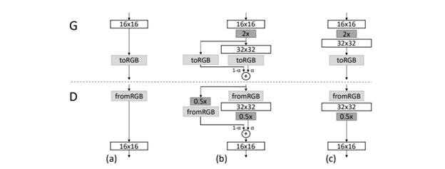
Figure 2. When doubling the resolution of the generator () and discriminator (), the new layers are faded in smoothly. This image illustrates the transition from 16×16 images (a) to 32×32 images ©. During the transition (b) they treat the layers that operate on the higher resolution like a residual block, whose weight increases linearly from 0 to 1.
2.1. Increasing variation
GANs tend to only capture a subset of the variation found in the training data. To improve this, Salimans et al. [2] suggested “minibatch discrimination” as a solution. In this method, instead of capturing only a subset of variation found in the training data, they computed feature statistics from both the images and minibatches, that leads the mini-batches of generated and original images to show similar feature statistics. This is implemented by adding a minibatch layer to the end of the discriminator in PGGAN that does not have any learnable parameters or hyperparameters. They computed the standard deviation for each feature in each spatial location over the minibatch and then averaged them over all features and spatial locations to make a single value.
2.2. Normalization
GANs are prone to the escalation of signal magnitudes as a result of unhealthy competition between the two networks (generator and discriminator). Most of the earlier solutions tried to solve this problem by using variants of batch normalization in the generator, and often in the discriminator. In this research, the authors used a different approach, without any learnable parameters, and consisting of two main components. The two components are:
-
A trivial, normal, random initialisation instead of a careful initialisation regime.
-
Scaling the weights dynamically in the runtime. This is a corrective to the scale invariance introduced by optimizers such as Adam. Each weight is normalized by a per-layer constant such that the weight updates are proportional to the weight magnitudes, effectively equalizing the ‘learning speed’ for all weights.
Moreover, they used the pixel-wise feature vector normalization in the generator to disallow the scenario where the magnitudes in the generator and discriminator spiral out of control as a result of competition. They normalized the feature vector in each pixel to unit length in the generator after each convolutional layer using a variant of “local response normalization” shown in Equation 1.

(1)
where , is the number of feature maps, and and are the original and normalized feature vectors in pixel , respectively.
3. Evaluation Metric
The authors used two metrics to evaluate the proposed method, multi-scale structural similarity (MS-SSIM), and the modified version of the Wasserstein distance called sliced Wasserstein distance (SWD).
MS-SSIM finds that the large-scale mode collapses reliably, but fails to assess image quality in terms of similarity to the training set, and also smaller effects such as loss of variation in colors and textures.
SWD indicates that the distribution of the patches is similar. It means that the training images and generated samples appear similar in both appearance and variation at this spatial resolution.
4. Experiments
In Table 1, the authors calculated SWD and MS-SSIM metrics for different configurations of their method and compared it to [3] on CELEBA and LSUN bedroom datasets.
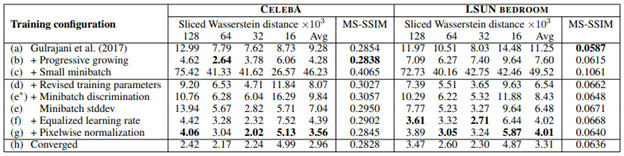
Table 1. Sliced Wasserstein distance (SWD) between the generated and training images and multi-scale structural similarity (MS-SSIM) among the generated images for several training setups.
Also, the generated images on CELEBA dataset using the above configurations are shown in Figure 3.
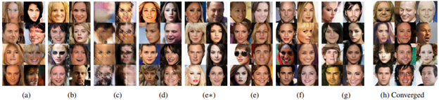
Figure 3. (a)-(g) CELEBA examples corresponding to rows in Table 1.
Moreover, the authors created a high-quality version of the CELEBA dataset consisting of 30000 images at 1024×1024 resolution and called it the CELEBA-HQ dataset. Figure 4 shows high quality generated images using this dataset. To generate these images, they trained the network on 8 Tesla V100 GPUs for four days. Table 2 shows the generator and discriminator structures to generate these samples.
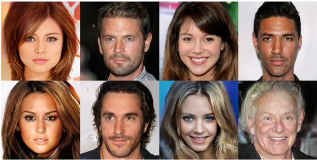
Figure 4. 1024×1024 images generated using the CELEBA-HQ dataset.
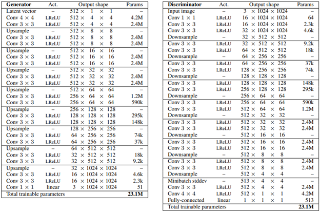
Table 2. Generator and discriminator used with CELEBA-HQ
Also, they generated images from different classes of LSUN dataset that are shown in Figure 5.
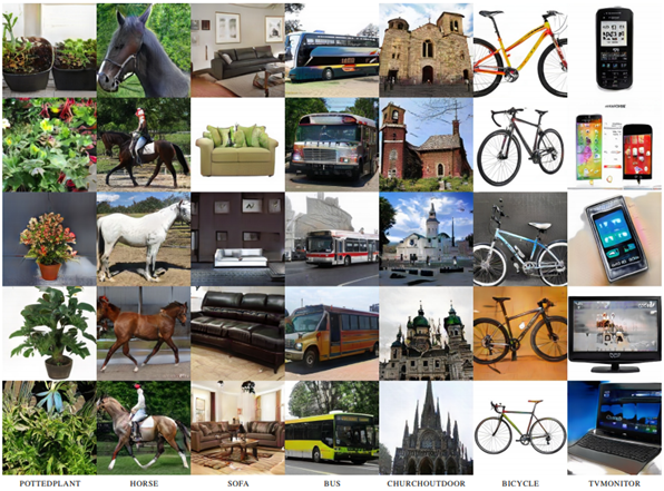
Figure 5. 256×256 images generated from different LSUN categories.
5. Conclusion
In this paper, the authors proposed a progressive GAN method to achieve high-resolution image generation. They started from one low-resolution generator and discriminator, then added one layer to both of them in each step which means the layers are gradually added . Moreover, they proposed some fading, minibatch variation, and normalization techniques to generate more real and high-resolution images.
To evaluate their method, they created a high-resolution version of CELEBA dataset (CELEBA-HQ) and generated new images using this dataset. Also, they use CELEBA and LSUN datasets to generate new images.
References:
[1] PGGAN paper: https://arxiv.org/pdf/1710.10196.pdf
[2] Tim Salimans and Diederik P. Kingma. Weight normalization: A simple reparameterization to accelerate training of deep neural networks. CoRR, abs/1602.07868, 2016.
[3] Ishaan Gulrajani, Faruk Ahmed, Mart´ın Arjovsky, Vincent Dumoulin, and Aaron C. Courville. Improved training of Wasserstein GANs. CoRR, abs/1704.00028, 2017.
Evolutionary Generative Adversarial Networks
Author: Alice Rueda| Author | Contribution |
|---|---|
| Alice Rueda | AR solely contributed to this section |
EGAN is based on Darwin’s evolution theory of “survival of the fittest”. In the context of GANs, this suggests that a model evolves as the environment (input) changes. In this sense, a member of a group of GANs will not be eliminated if it has a higher likelihood of generating more diverse output with the given inputs. As the members are evolving, the comparatively “unfit” ones, i.e., the ones that generate limited variations (such as mode collapse or close to) will be eliminated.
Variation Through Mutation
As the discriminator evolves during the training process, the update in the model provides an ever-changing environment for the generators to be adapted. Each generation (iteration) of the generators will undergo a mutation as the evolution mechanism. The offsprings are duplicates of the parents (asexual reproduction) with variations. The evolution, in a sense, changes the parameters of the networks. The performance of the generators is measured based on the quality and diversity of the generated samples. Poorly performed generators are eliminated.
The mutation has three parts. There are two complementary mutation operations (the lost function of the generator), minimax mutation () and heuristic mutation (), and a least-square mutation (). The minimax mutation minimizes the log probability of discriminator being correct. The heuristic mutation maximizes the log probability of the discriminator being fooled. The least-square mutation measures the L_2 norm of the probability of the discriminator being fooled to always wrong.
Evolution Through Performance Measure
The performance (fitness) of the generator is measured based on quality () and diversity (). The quality fitness score measures how well the generator fools the discriminator. The log gradient of updating the discriminator is used as the diversity measure. Small discriminator gradients tend to have spread out (more diverse) generated samples. With a balancing factor 𝞬, the overall fitness score is .
Experiment
The platform used to run the model is an Alienware with 16 GB memory and a 1060 GPU. If you are running on your PC with a GPU, you need to go through the following settings and changes.
Some issues have been created on Github for the author to fix them. https://github.com/WANG-Chaoyue/EvolutionaryGAN-pytorch/issues
Package installation
- Requirement.txt lists the minimum version of the packages. However, scipy has deprecated imread() in version 1.3.0. To run the code, you need to install an older version such as scipy==1.1.0 listed on the requirement.txt. With pillow install, image manipulation will work.
The list of package versions under conda environment are:
Pytorch = 1.0.0
Torchvision = 0.2.1
Dominate = 2.4.0
Visdom = 0.1.8.8
Numpy = 1.17.1
Scipy = 1.1.0
H5py = 2.9.0
Pillow = 6.1.0
Tqdm = 4.35.0
- The readme.md file says to initialize the *.npz file. You will also need to download the inception model and prepare the *.npz file. This is to evaluate the GAN using inception moments. You can use the sample python code to generate C10_inception_moments.npz in the /inception_pytorch directory and copy the file to the required directory/filename:
python inception_pytorch/calcuate_inception_moments.py --dataset C10 --data_root datasets
copy C10_inception_moments.npz to /TTUR/stats/fid_stats_cifar10_train.npz
NOTE: Make sure your cudatoolkit package version matches your cuda driver version and pytroch version. You can check your driver version on the command line **nvidia-smi **or nvcc --version.
Code modification
-
Base_model.py: line 80-83 comment out tensorflow GPU usage configuration code (since this is not needed for pytorch), or you can add import tensorflow as tf.
-
Base_options.py: (This modification has already included in the training script. You might not need to change this. This is for your information to what to change if you want to use other base network instead of DCGAN. Then you will also need to add the model in the model directory.)
-
line 38 change the default netG model from ‘resnet_9blocks’ to ‘DCGAN_cifar10’. The only model included in the model set and defined in the network.py code is ‘DCGAN_cifar10’. The easiest to fix this is to change the netG default setting.
-
Line 37 change netD model from ‘Basic’ to ‘DCGAN_cifar10’.
Training
To start train, simply run the script file as:
bash ./scripts/trian_egan_cifa10.sh
The script will automatically download the cifar-10 images before training. This might take a while. If you already have the cifar-10-python.tar.gz file, you can comment out the line and the tar.gz file to ./datasets/cifar10 directory.
Unfortunately, the 1060 GPU is not powerful enough to complete the training in a reasonable amount of time. Since the code uses older packages, there were a lot of warning messages. The execution also displayed tensorflow core, stream_executor and compiler information followed by the options as in Figure 5.1. The execution was terminated of epoch_15 with the training output showing:
Files already downloaded and verified

dataset [TorchvisionDataset] was created

The number of training images = 50000

initialize network with normal

initialize network with normal

model [EGANModel] was created

---------- Networks initialized -------------

[Network G] Total number of parameters : 12.654 M

[Network D] Total number of parameters : 11.033 M

create web directory ./checkpoints/egan_cifar10/web...

(epoch_1) End of giters 130 / 500000 Time Taken: 355 sec
(epoch_2) End of giters 260 / 500000 Time Taken: 352 sec
(epoch_3) End of giters 390 / 500000 Time Taken: 353 sec
(epoch_4) End of giters 520 / 500000 Time Taken: 354 sec
(epoch_5) End of giters 650 / 500000 Time Taken: 353 sec
(epoch_6) End of giters 780 / 500000 Time Taken: 356 sec
(epoch_7) End of giters 910 / 500000 Time Taken: 519 sec
(epoch_8) End of giters 1040 / 500000 Time Taken: 353 sec
(epoch_9) End of giters 1170 / 500000 Time Taken: 353 sec
(epoch_10) End of giters 1300 / 500000 Time Taken: 354 sec
(epoch_11) End of giters 1430 / 500000 Time Taken: 353 sec
(epoch_12) End of giters 1560 / 500000 Time Taken: 779 sec
(epoch_13) End of giters 1690 / 500000 Time Taken: 947 sec
(epoch_14) End of giters 1820 / 500000 Time Taken: 352 sec
(epoch_15) End of giters 1950 / 500000 Time Taken: 353 sec
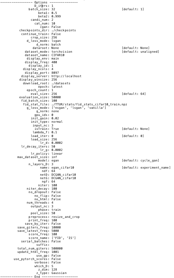
Figure 5.1: Execution options display for EGAN training.