Anomaly Detection; An Overview
Contributors: Alec RobinsonEric Djona FegnemHarriet YuLindsey PengMichael EnquistPeter BacalsoRamya BalasubramaniamSamantha CassarVictor ReyesWilly RempelYenson Lau
Editors: Chris BobotsisSusan Shu Chang
This blog post is the collective work of the participants of the Anomaly Detection workshop organized by Aggregate Intellect. This post serves as a proof of work, and covers some of the concepts covered in the workshop in addition to advanced concepts pursued by students.
Table of Contents
Introduction
Author: Willy Rempel| Author | Contribution |
|---|---|
| Willy Rempel |
Introduction
An anomaly is by definition something that is outside the norm or what is expected. For data this can mean rare individual outliers or distinct clusters. Anomaly detection is an important capability with broad applicability in many domains such as medical diagnostics or in detection of intrusions, fraud, or false information. All three categories of model training are used for anomalous data; supervised, semi-supervised, and unsupervised. Typically the first go-to methods are statistical and classical machine learning techniques. These can be low cost and yet very effective. When the data is more complex, deep learning approaches are required to extract the relevant latent features.
Basic statistics of the data distribution, such as the standard deviation, can be immediately used to identify outliers (e.g. anything further than from the mean). Boxplots visually show possible anomalies at the tail ends of plot whiskers. More advanced methods such as Gaussian mixture models (GMM) provide a generative model to discriminate outliers from more complicated distributions. These methods assume a parametric distribution. Non-parametric techniques include histogram based outlier score (HBOS) and distance-based (clustering) techniques, such as -nearest neighbours (-NN) and local outlier factors (LOF).
The HBOS is produced by taking the product of the inverse histogram values for each feature of a sample. It is fast at the cost of less precision and is better suited for detecting global outliers vs. local ones. There are several options for using (-NN), starting with a simple 1-NN where we score based on the distance from the closest neighbour. We could also score based on the average distance to k neighbours. LOF elaborates on -NN by using the neighbourhood density of samples. First, the inverse local neighbourhood density, or local reachability desnity (LRD), of a sample is computed as
The LRD is computed for all neighbours of and used for the final LOF score, which is a ratio of the neighbourhood density of with respect to the densities of its neighbours.
Other clustering techniques used for anomalies are:
- -means
- hierarchical clustering
- density-based spatial clustering of applications with noise (DBSCAN)
- cross interaction based outlier score (XBOS)
- cluster-based local outlier factor (CBLOF, uCBLOF), a clustered variant of LOF.
Isolation forests (iForest) are an ensemble of isolation trees where instances are isolated based on random selection of features and feature values for decision splits. Anomalies will be more susceptible to isolation and will have shorter average paths (averaged over all the decision trees). As the name suggests, One-SVM (support vector machine) creates a decision boundary around only one class: the set of all normal data. Any anomaly will lie outside the boundary. The advantage of one-class modelling is that we do not need to know about and account for every possible anomaly. Instead we accurately model as much as possible what ‘normal’ means for the data. Additionally we can use semi-supervised techniques such as data shuffling to generate fake/shuffled samples to better learn the decision boundary.
One-class classification also works very well for deep learning models. Autoencoders (AE) trained on normal data will have high reconstruction error scores for anomalous instances. The same is the case for any generative models which will learn the distribution of normal data. Variational autoencoders (VAE) can also utilize the KL-divergence score of an instance to indicate how unlikely is the data from the learned distribution. Adversarial autoencoders (AAE) add a discriminator to a VAE which discriminates between the instance latent embedding and some previously selected task-specific distribution.
GANs are another obvious choice where the discriminator from a trained GAN is used to detect outliers. Conditional GANs refine this by including conditional class labels to both the generator and discriminator. This is preferable as it favours the generator in the game, resulting in better discriminators. The first example of a conditional GAN is a repurposed VAE. The VAE is used for the generator and the condition is the input data itself. Both the actual and reconstructed data are sent to a discriminator. The generator is still used during inference, as any anomalous data will be poorly reconstructed, increasing the likelihood of a true positive. Adversarial Dual Autoencoders (ADA) takes this a step further and uses another VAE for the discriminator. GANomaly combines a VAE with the encoder half of another VAE, and also some other discriminator. This leaves us with three scores to work with:
- : The loss between the two latent embeddings of the generator VAE and the 2nd encoder
- : The normal VAE reconstruction loss
- : A binary real/fake score from the 2nd discriminator
Deep learning has the additional benefit of being able to work with sequential data using auto-regressive models and RNNs. Such models assign probabilities to sequence elements and can spot single element or whole sequence anomalies. Lastly, deep hybrid models combine both deep learning and prior techniques. For example, the latent code book of an autoencoder can be extracted and have -NN applied for clustering the codes.spot single element or whole sequence anomalies.
Next, we advanced techniques presented in three papers. The first paper, Temporal Cycle-Consistency Learning, uses the cycle-consistency concept to align sequential data streams where there is some natural correspondence between the two sequences. An example is videos of pouring water from a pitcher. The second paper covered is GLAD: GLocalized Anomaly Detection via Active Feature Space Suppression. A neural network is used to modulate the output of LODA, an ensemble method for anomaly detection. Additionally, active learning is used in the training loop. Lastly we have Unsupervised Anomaly Detection with Generative Adversarial Networks. A one-class technique is applied to medical images with AnoGAN; a generative adversarial network that learns the distribution of healthy tissue images.
Temporal Cycle-Consistency Learning
Author: Ramya BalasubramaniamAuthor: Yenson LauAuthor: Alec Robinson| Author | Contribution |
|---|---|
| Ramya Balasubramaniam | Drafted the related work & applications, dataset & evaluation, experiments, and conclusion sections. |
| Yenson Lau | Drafted the introduction, related work & applications, and theory sections. Revised and edited all remaining sections. |
| Alec Robinson | Contributed to the theory section. |
Introduction
Temporal cycle consistency (TCC) learning is a self-supervised method that aligns videos and general sequential data by learning an embedding to capture correspondences across videos of the same action.
Compared to existing methods, TCC learning does not require explicit alignment information between sequences (which are hard to acquire), and can handle significant variations within an action category. The learned embeddings also appear to be useful for fine-grained temporal understanding of videos and action parsing, suggesting that rich and useful representations can be learned simply by looking for correspondences in sequential data.
Features and Applications
Although cycle consistency is conventionally used to find spatial correspondences for image matching and co-segmentation tasks, this work switches the emphasis to temporal consistency and presents a differentiable cycle consistency loss for self-supervised learning.
This allows the TCC model to optimise over pairs of videos to encourage cycle consistent embeddings for sequences of the same action. Compared to previous video alignment or action parsing techniques, this is a simpler approach that removes the need for manual labelling and other types of synchronisation information, that are usually difficult to acquire.
The embeddings obtained by this method are rich enough to be useful for a variety of tasks. One clear application that TCC allows is to synchronise the pace at which an action is played back across multiple videos. This alignment also enables cross-modal transfer; for example, the sound made when pouring a glass of water can be transferred from one video to another solely on the basis of its visual representation. Since the embedding is so effective at isolating the action from the training data, learned TCC representations allow for fine-grained retrieval in videos, such as differentiating before and after frames of baseball pitches depending on the positioning of the pitcher’s legs alone.
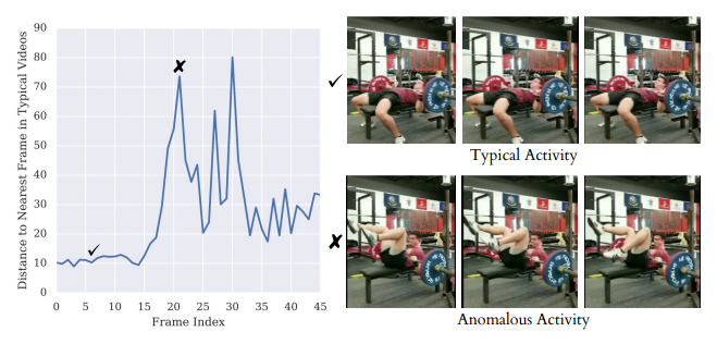
Finally, TCC learning can also be used to generate features for anomaly detection. When TCC is used to learn embeddings of video sequences of some typical behaviour (e.g. videos of bench presses), embeddings of new sequences will deviate from typical trajectories whenever anomalous activities occur.
Cycle Consistent Representation Learning
Assume that we are given two video sequences and with lengths and , respectively. Their embeddings are computed as and s.t. and , where is the neural network encoder parameterised by . The goal is to learn an embedding that maximises the number of cycle consistent points* for any pair of sequences in from the data:
Cycle consistency. A point is cycle consistent iff , where . We call the cycle-back of .
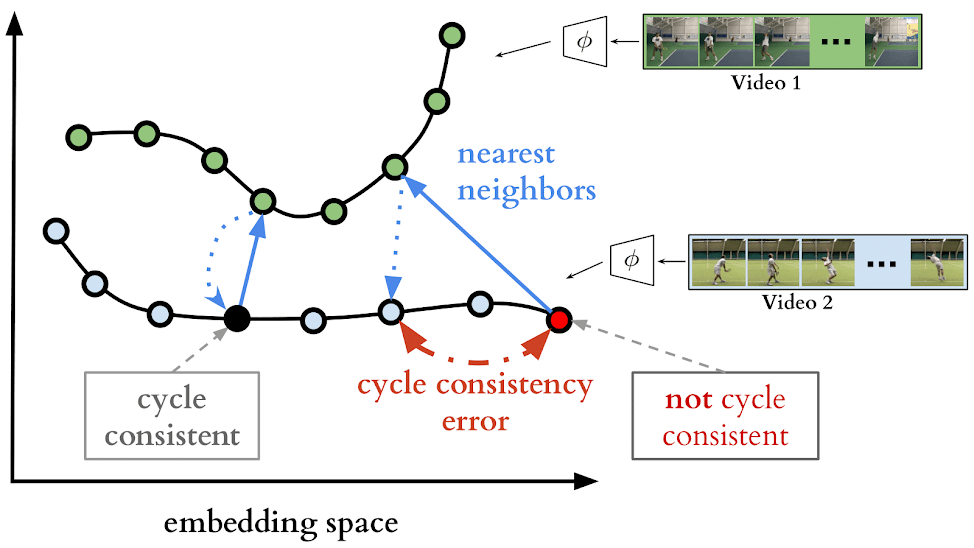
In other words, is cycle consistent if taking the nearest neighbour to from , then finding the nearest neighbour back to , returns the same point .
By maximising the cycle consistency of sequences describing a specific action, our embedding space captures the common structure across the videos in our dataset (i.e. the action itself) despite the presence of many confounding factors present between videos, such as angle and location.
Differentiable Cycle-back
To perform optimisation, this work presents a differentiable cycle-back procedure, which starts from by computing the softmax values
,
so that is a similarity distribution on . Correspondingly, the soft neighbour to is given by . We cycle back to by computing
,
so that is a similarity distribution on .
Then is updated (through the embedded points and ) to minimise two loss functions:
The cycle-back classification (cbc) loss is given by the cross entropy between and the truth distribution , where the correct entry has value 1 and all other entries are zero:
.
The CBC loss measures the ability of to be classified to the correct cycle-back point .
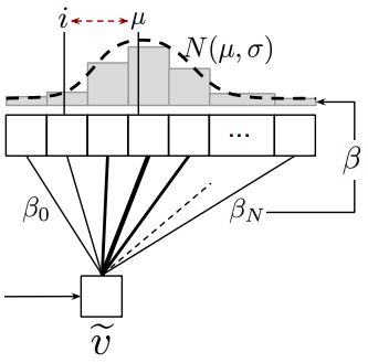
The cycle-back regression (cbr) loss encourages to concentrate around the -th entry by penalising based on its mean location as well as its variance :
.
Here and , and is a trade-off parameter between the location and variance penalties.
Implementation Details
Training procedure. Sequence pairs are randomly picked from the dataset. For each sequence pair, optimization is done stochastically by picking a random frame and descending on , picking frames randomly until convergence.
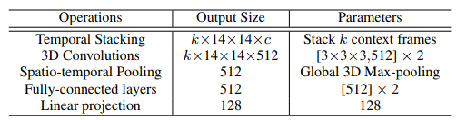
Encoding network. All frames in a given video sequence are resized to . Image features are then extracted from each frame using either pretrained features extracted from the Conv4c layer of ResNet-50, or from a smaller model to be trained from scratch, such as VGG-M. The resulting convolutional features have size , where is either 1024 or 512 depending on whether ImageNet or VGG-M is used.
The image features of each frame are stacked with those of other context frames, and 3D convolutions are applied to aggregate temporal information. This is followed by 3D max pooling, two fully-connected networks, and a linear projection layer to produce the final embedding space, which has dimension ; details are shown in the adjacent table.
Evaluation
Three evaluation measures are used to evaluate fine-grained understanding of the model on a given action. TCC networks are first trained and then frozen. SVM classification and linear regression is performed on the features from the networks, with no additional fine-tuning of the networks. Higher scores indicate better performance for each measure:
-
Phase classification accuracy: Whether the TCC features allow the correct phase to be identified by training an SVM classifier on phase labels of the training data.
-
Phase progression: How well the “progression” of a process or action was captured by the embedding. Progression is measured as the fraction of time-stamps passed in the current frame between key events. Linear regression is applied to predict progression values on TCC features. Performance is computed as the the average R-squared measure,
,
where is the ground truth progress value, is the average of s and is the prediction made. The maximum value of this measure is 1.
-
Kendall’s Tau is a statistical measure that determines how well-aligned two sequences are in time, and does not require additional labels for evaluation. For a pair of videos, each pair of embeddings in the first video are used to retrieve their nearest embeddings in the second video, . This quadruplet of frame indices are said to be concordant if and or and ; otherwise they are discordant. Kendall’s Tau is then calculated over all embedding pairs from the first video,
.
Here denotes the length of the first sequence and the denominator represents the total number of pairs present in the first video. A value of 1 implies that videos are perfectly aligned, while a value of -1 implies that the videos are aligned in reverse.
When is averaged over all pairs of videos in the validation set, it serves as a measure of how well TCC learning generalizes for aligning new sequences. It assumes, however, that there are no repetitive frames in a video, and may not accurately reflect desired performance when videos taken involve slow or repetitive motion. Neither of these issues are present in the datasets used for this work.
Experiments
Baselines
TCC was compared with existing self-supervised video representation learning methods:
- Shuffle and Learn (SaL): Triplets of frames are randomly shuffled and a small classifier is trained to predict if the frames were in order or shuffled. The labels for training this classifier are derived from the indices of the triplet sampled. This loss encourages representations that encode information about the order in which an action should realistically be performed.
- Time-Contrastive Networks (TCN): frames are sampled from the sequence and used as anchors (in the sense of metric learning). For each anchor, positives are sampled within a fixed time window, resulting in -pairs of anchors and positives. The -pairs loss considers all other possible pairs as negatives. This loss encourages representations to be disentangled in time while still adhering to metric constraints.
- Combined Losses: The cycle consistency loss can be combined with all SaL and TCN losses to get more training methods. The authors learn embeddings using and , where is chosen by searching from the set . The video encoder architecture remains the same.
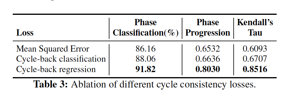
Ablation of Different Cycle Consistency Losses
The phase classification, phase progression, and Kendall’s Tau metrics were measured on the Pouring data set using TCC features trained on either the cycle-back classification (CBC), cycle-back regression (CBR) or mean square error (MSE) losses exclusively. The MSE loss is equivalent to the CBR loss without variance penalization, i.e. . Based on the results below, the CBR loss with outperforms all other losses, and is used for the remaining experiments.
Action Phase Classification
Self-supervised learning with trained vs. fine-tuned encoding networks. The authors compared phase classification results when TCC features were learned on either a) a smaller VGG-M encoder network trained from scratch, or b) a fine-tuned, pretrained ResNet-50 network.
Using TCC features for phase classification appears to be generally superior to a supervised classification approach, regardless of the choice of encoder network. This is expected since there are few labels available in the training data. With the VGG encoder, TCC features provided the best phase classification results regardless of dataset. This might be attributed to the fact that TCC learned features across multiple videos during training but SaL and TCN losses operated on frames from a single video only.
The scarcity of training data also means that features trained on the fine-tuned ResNet-50 encoder generally achieve higher performance, and are used for all remaining experiments. In this case, SaL, TCN, and TCC each are able to yield competitive features for phase classification. For the Pouring dataset, TCC features yielded the best performance, whereas TCC + TCN yielded the best performance on the Penn Action dataset. The authors speculate that the combination of losses may have reduced overfitting in the latter case.
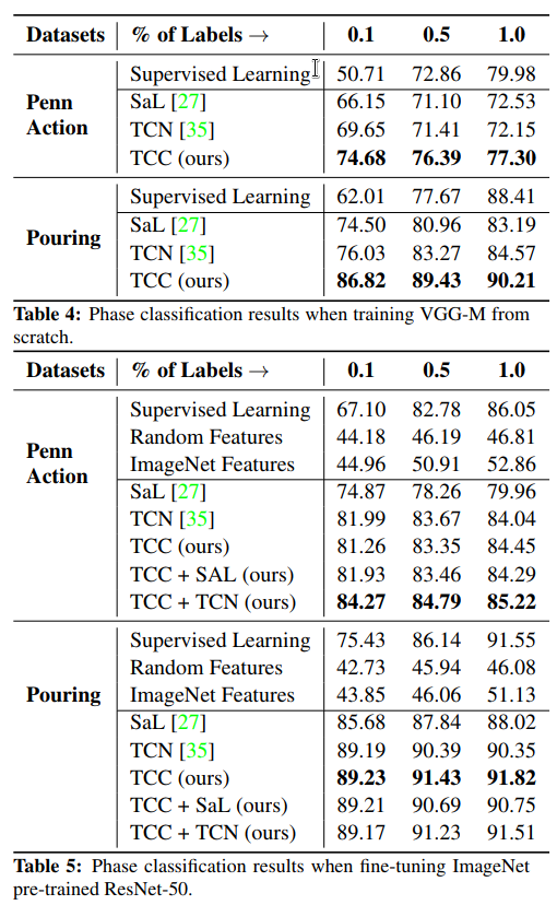
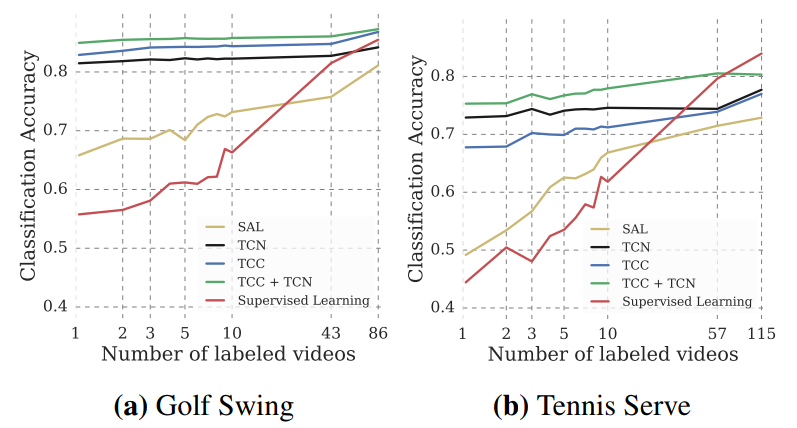
Self-supervised Few Shot Learning. In this setting, many training videos are available but per-frame labels are only available for a few of them – in this case, each labelled video contains hundreds of labelled frames. Self-supervised features are learned on the entire training set using a fine-tuned ResNet-50 encoder. These are compared against features extracted using supervised learning on videos for which labels are available. The goal is to see how phase classification accuracy increases with respect to the number of labelled videos. Based on the results on the Golf Swing and Tennis Serve videos from the Penn Action dataset, TCC + TCN features are able to extract enough information to outperform supervised learning approaches until roughly half the dataset is labelled. This suggests that there is a lot of untapped signal present in the raw videos which can be harvested using self-supervision techniques.
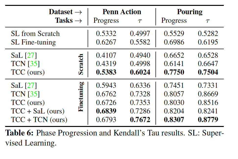
Phase Progression and Kendall’s Tau
The remaining tasks measure the effectiveness of representations at a more fine-grained level than phase classification. In general, features obtained using TCC alone or in combination with another self-supervised loss leads to best performance in both tasks. Moreover, significantly higher values for Kendall’s Tau are obtained with features extracted TCC + TCN losses.
Conclusion
The TCC method was able to learn features useful for temporally fine grained tasks. In multiple experiments, it is observed that TCC, being a self-supervised method, enjoyed significant performance boosts when there is a lack of labelled data. With only one labelled videos, TCC achieved similar performance to existing supervised learning models trained with roughly 50 labelled videos. Based on its numerous possible applications, TCC can serve as a general-purpose temporal alignment method that works without any labels, benefiting any task which relies on alignment.
GLAD: GLocalized Anomaly Detection via Active Feature Space Suppression
Author: Victor ReyesAuthor: Lindsey PengAuthor: Michael EnquistAuthor: Harriet Yu| Author | Contribution |
|---|---|
| Victor Reyes | Drafted Method section and loss function subsection. |
| Lindsey Peng | Drafted Introduction, Method, and Active Learning in the FSSN subsection. |
| Michael Enquist | Drafted Introduction section, contributed to Experiment, and Conclusion sections. |
| Harriet Yu |
1. Introduction
GLAD (GLocalized Anomaly Detection) incorporates an active learning for anomaly detection by applying an ensemble via neural network approach to anomaly detection. The algorithm learns and retrains from the global and local feature space by the local labelled instances in the dataset. The active learning method in this approach is to capture the total number of correct anomalies and presented to the analyst. Then, the analyst labels the instance, and the anomaly detector updates its model from the newly acquired instance labels. By applying a neural network, this dynamically changes the weights of each anomaly detector scores based on the input data. The input data is fed to both the ensemble and the Neural network and an ensemble of M anomaly models. M models output M anomaly scores, and the neural network output M probabilities corresponding to the relevance of each model given the input data. The anomaly scores and their corresponding probabilities are multiplied and combined to provide the Final Anomaly Score. The ensemble detectors are not updated, the neural network is updated through gradient descent with the error from the loss function.
Based on previous work, GLAD applies a Lightweight Online Detector of Anomalies (LODA), which is an ensemble system for detecting feature space variables and rank the features of each member (Pevný, 2015). The algorithm uses a neural network which is pre-trained on the unlabelled instances, and tuned to adjust the local relevance of each ensemble member using all labelled instances. As well, GLAD is previously related to Active Anomaly Detection (AAD), which is an expert feedback system for adjusting to the anomaly detection outliers and hyper tunes with the analyst’s understanding of the anomalies (Shubhomoy Das, 2016). AAD is a lighter and simpler version of Rare Category Detection (RCD) as it requires only labelled instances rather than having K distinct existing or unseen classes (Shubhomoy Das, 2016). In each iteration, this algorithm selects an instance of potential anomaly outliers for the end-user. Then, the end-user or human analyst will label the outliers as an anomaly or not (Shubhomoy Das, 2016).
2. Method
Training:
- The neural network(Feature Space Suppression Network AKA FSSN) is first initialised with weights by training it to output uniform probability for all unlabeled data. This is called priming.
- Active learning is performed by having the network train over the whole dataset and presenting the top percentile most anomalous data points to an expert analyst for labelling.
- Step 2 is repeated as many times as desired. Eventually the entire dataset would be labelled, but ideally a middle ground is reached where the analyst only has to label a small amount of data to achieve good results.
Loss Function
The loss function used by GLAD can be seen below, and is composed of two parts: the first term represents the active learning portion, while the second term is used to provide a “prior” over the dataset.
The second term is easier to understand, so we will start there:
-
is a hyper-parameter used to tune the relative importance of the two terms in the loss function. In the paper they have set it to be 1 for all their experiments.
-
D is set comprising the entire dataset. This means that the second term is really the mean of over D. is the total number of elements in D.
-
is the mean binary cross entropy over a hyper-parameter b, and the importance the network is assigning to x for each detector. The authors of the paper do not give a particular value of b to use, but we believe that setting b to be , where is the number of detectors, would be optimal.
In all this second term is trying to bring all the importance the network computes to some value b. They call this a “prior”. In that sense they assume that given no other information, each detector in the ensemble should have equal importance. They claim that this is a good starting point for active learning.
The first term in the loss function is more complicated and requires a bit more notation to set up. is the set of data points (feature vectors and labels) that have been labelled by an expert up to iteration t. This means that the first term is really the mean of over that set of labelled points.
Aside: It seems like there is a small typo in the paper at equation 3, the definition for . It lists this loss as being the sum of the two terms, but it turns out that both of those terms are equivalent. The authors state later in the paper that . If one were to implement the equations as they’re written the network would still learn, but the loss being calculated for the first term of the overall loss equation would be double. As it stands this typo is merely typographical and does not negatively impact the results of the paper.
Here we see a modified form of hinge loss: if is negative we don’t want to have any gradients to propagate through the FSSN. The terms in this expression are as follows:
- Score is the output of the network as a whole; that is +1 for an anomaly and -1 for a normal value. That means that Score(x) is the final output of the network for some input vector x.
- is the Score of the 'th percentile based on the labelled data points up until iteration t-1. We can think of as expressing our belief over how much contamination exists in the dataset. The higher is the lower contamination we believe is in the dataset.
- y is the expert defined target which is one of +1 for an anomaly and -1 for a normal data point.
Now we see that if Score(x) is greater than , the network is telling us that x is probably one of the anomalous points. This would make the value in the brackets negative. If the expert has also agreed that x is anomalous, then we will multiply this value by +1 and the network will not have to change its prediction for this data point. However, if this was actually a normal value (-1) then we will generate a loss that the network will have to minimise by reducing the value of Score(x).
If Score(x) is less than , the network is telling us that x is probably one of the normal points. This makes the term in brackets positive, which if the network and the expert agree means we get a negative number which leads to no loss. If the network and the expert disagree we will get a loss that is reduced by increasing the value of Score(x).
Putting the above cases together, we can see that the loss function only assigns a loss when the expert and the network disagree. Any time the two are in agreement, no update is made to the network.
So overall can be understood as assigning a loss when the expert and the network disagree, but also having a background component trying to make the contribution of all the detectors about equal. In a sense the network should only deviate from this equal relevance across the detectors if it believes that it will lead to a better outcome.
The Idea of Active Learning Employed in the Feature Space Suppression Networks:
An Active learning strategy is usually adopted when labelled data is not readily available. Its steps generally include:
-
Having only a subset of the available data labelled by a human-being and leaving labels of rest of the data to be inferred by the model trained on the labelled data
-
Iterate by evaluating the model trained, if not qualified, then extract a new subset of data and label manually and retrain the model
As the following graph describes in the authors’ other paper “Active Anomaly Detection via Ensembles: Insights, Algorithms, and Interpretability”:
In particular, in the batch active anomaly detection learning framework (BAL) in this paper, for each iteration, assume a human analyst can label a size of b data points:
- The unlabelled data point enters the FSSN and generates a relevance score per detector in the ensembles, so it is a score that describes detectors per input and a cross-entropy function evaluates the quality of the relevance scores.
- Ask the available human analyst that can provide information on the label of the data point just input.
- Each detector of the ensemble then generates a score for the data point inputted, higher for assuming anomaly, lower otherwise, and this result is evaluated against a threshold q, that which a good result should be higher.
- The quality of the entire system is a combination of step 1 and 3 given by the feedback information incorporated in step 2 by a human analyst and then average out all iterations.
Discussion
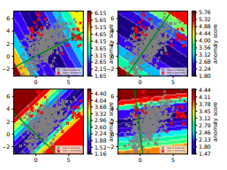
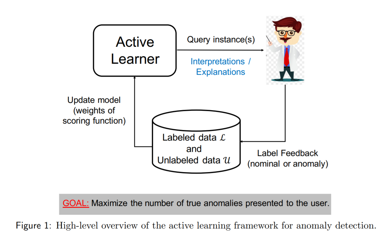
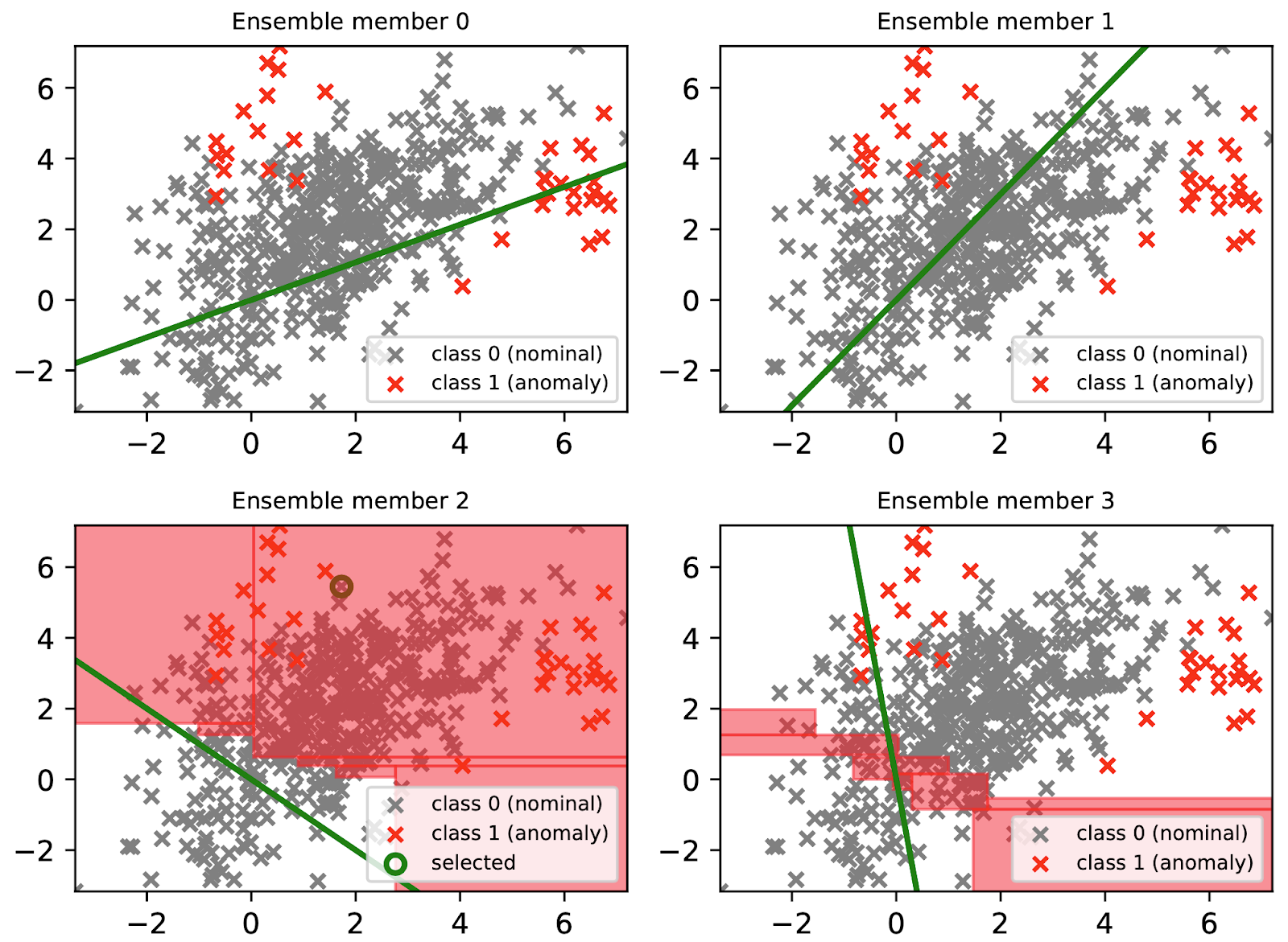
Figure 1. Colours represent anomalies
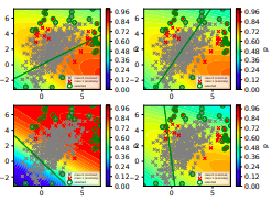
Figure 2. Colours represent relevance. (Shubhomoy Das, 2016)
Traditional methods gives global weights to detectors, even though they may only be useful in a particular feature space. Figure 1 shows the problem with using global weights for the four anomaly detector models from LODA ensemble detectors. Only the bottom left model is somewhat accurate for the global set. You can see that when the points are projected on the bottom left line, the normal data falls mostly in the center of the detector while the anomaly scores are separated at the two ends of the line(just like a normal distribution with anomalies happening at two ends of the distribution). This means that the other 3 models are counter-effective for the anomaly detection for most data points in different data spaces.
In comparison, this paper learns the relevance (Figure 2) of each of the four models from LODA depending on the data. Overall, the neural network learns to suppress the signal of the models when it is irrelevant and vice versa.
By weighing the individual models with their relevance in different feature space, GLAD was shown to detect anomalies for 7 different datasets.
3. Experiment
In order to reproduce similar results from the paper, the author has provided the code on GitHub. The following commands apply for the GLAD algorithm on the Toy dataset:
python -m ad_examples.glad.glad_batch --log_file=temp/glad/glad_batch.log --debug --dataset=toy2 --n_epochs=200 --budget=60 --loda_debug --plot
If the explanation library LIME (Ribeiro et al. 2016) is installed then you can use the following command:
python -m ad_examples.glad.glad_batch --log_file=temp/glad/glad_batch.log --debug --dataset=toy2 --n_epochs=200 --budget=30 --loda_debug --plot --explain
This model can be run by using the following settings and changes:
- Tested with python 3.6.1, tensorflow = 1.6.
- Apply t-SNE (or any dimensional reductionality method) for the labelled dataset (most of the datasets in the repository are already reduced. )
- The
glad_batch.pyscript (~ad_examples-master/ad_examples/glad/glad_batch.py) needs to be modified if the user wants to apply the seven different datasets referenced in the paper (e.g Abalone, ANN-Thyriod, Cardiotocography, etc.) - For additional installation requirements, please read requirements.txt on GitHub.
Training results:
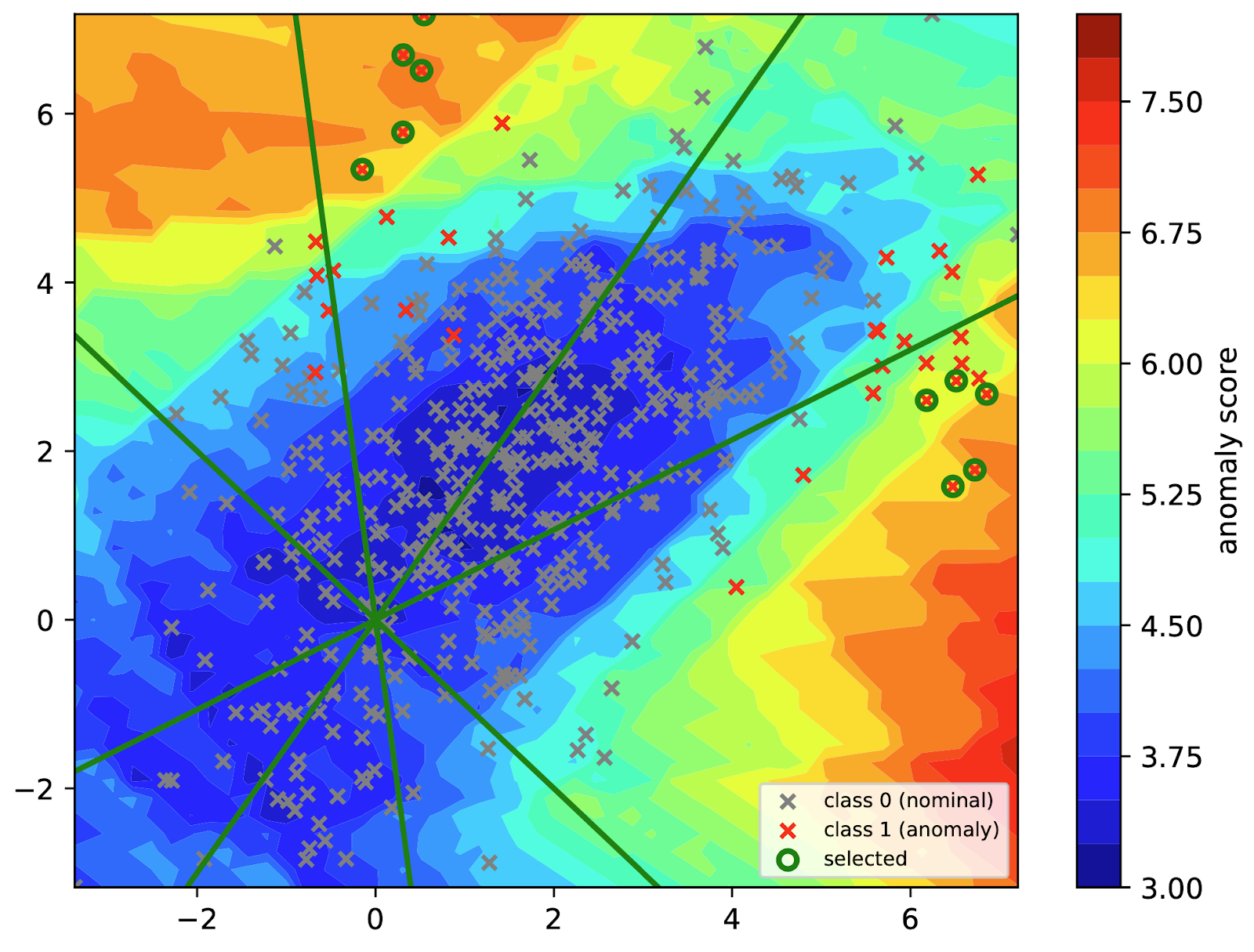
Here is the following training results figures represented from the Toy dataset:
Training Result Figure 3. Relevance after 30 feedback iterations
As we can see from Figure 3 (above), the visualisation reproduces similar decision boundaries from the paper and detecting the selected anomalies from the analyst.
Training Result Figure 4. Model Agnostic Explanation Technique (LIME)
The above Figure 4 is intended to provide relevance of a specific ensemble member (detector) in the feature space. In the paper discussion, GLAD assumes that the anomaly detectors in the ensemble can be arbitrary. The best it can offer as an explanation is the member which is most relevant for a test instance.
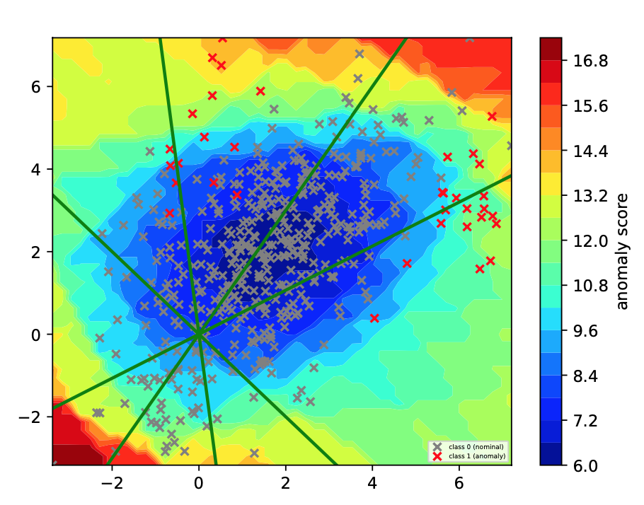
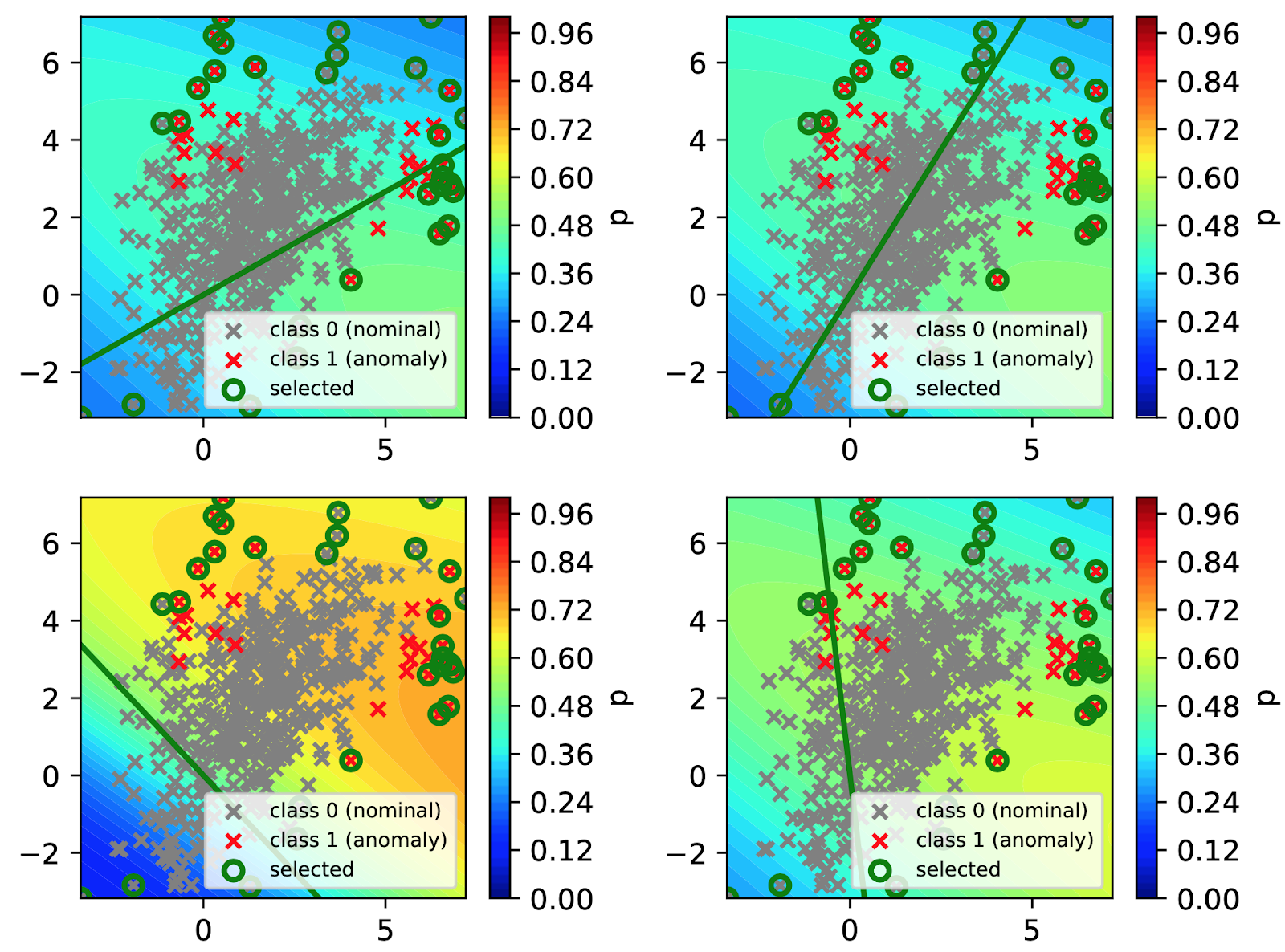
Training Result Figure 5. Comparing LODA score contours from the experiment vs the paper.
The above Figure 5 reveals the overall result from the LODA projections from the Toy dataset. Figure 5 results from the experiment( left ) and in the paper (right) were similar. The only difference is the anomaly score range, which shows the concentration of the score anomalies. Our experimental result was able to select the anomalies for the analyst. For instance, on the left diagram on Figure 5, shows 10 labels being selected, whereas on the right diagram (in the paper), there was none. Effectiveness and consistency are very important and based on the results from Figure 3 to 5; the model performs consistently well on the identification of the anomalies from the toy dataset.
4. Conclusion
We brought attention to an active learning approach to anomaly detection by incorporating expert feedback. The paper and experiment results demonstrated the practical usage of an expert feedback system for adjusting to the anomaly detection outliers. The next steps are to apply on various real-world datasets besides the seven datasets mentioned in this paper. It is important for having expert feedback for anomaly detection, especially if the outliers are inline with the experts’ idea of an anomaly.
Unsupervised Anomaly Detection with Generative Adversarial Networks to Guide Marker Discovery
Author: Eric Djona FegnemAuthor: Peter BacalsoAuthor: Samantha Cassar| Author | Contribution |
|---|---|
| Eric Djona Fegnem | Equal contribution. |
| Peter Bacalso | Equal contribution. |
| Samantha Cassar | Equal contribution. |
Introduction
Anomaly detection in imaging data is challenging. Current models typically rely on supervised machine learning approaches. Such models require a large amount of labeled data with known markers. Their quality depends upon their accuracy in correlating markers with disease status, and treatment response. While many diseases lack a sufficiently broad set of markers, others have markers with limited predictive power. Furthermore, models that rely on supervised approaches cannot detect novel makers. Here, the authors proposed AnoGan, an unsupervised learning model trained on imaging data capable of identifying anomalies. AnoGan is composed of a deep convolutional generative adversarial network that learn anatomical variability of healthy images and a novel anomaly scoring scheme based on the mapping from image to latent space. Results on optical coherence tomography (OCT) images of the retina demonstrate that the approach correctly identifies anomalous images, such as images containing retinal fluid or hyperreflective foci.
Deep Convolutional Generative Adversarial Networks
The authors used a deep convolutional generative adversarial network (DCGAN) to learn the manifold of normal anatomical variation. In DCGAN, the generator learns to generate 2D images. A GAN consists of two adversarial modules, a generator and a discriminator . During training, the GAN learns the variability of the training data in an unsupervised fashion, resulting in a learned manifold . The manifold consists of 2D images of healthy examples of OCT scans, which the generator G uses to map 1D vector samples () of uniformly distributed input noise sampled from latent space for a learned distribution (). The discriminator is a CNN that maps a 2D image to a scalar value representing the probability that the given input is a real image from the training set or is generated by the generator.
and are simultaneously optimized through a two-player minimax game with the following value function:
Here, the discriminator is trained to maximize the probability of correctly discriminating real training examples from generated samples from , while the generator is trained to fool the discriminator into labelling a generated sample as a real one. Through training, both modules become increasingly better at generating realistic images and in correctly identifying generated images, respectively.
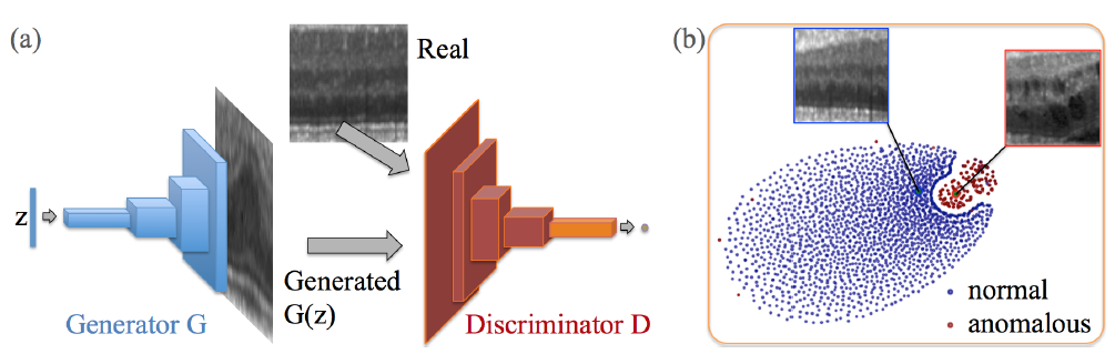
(a) Deep convolutional generative adversarial network. (b) t-SNE embedding of normal (blue) and anomalous (red) images on the feature representation of the last convolution layer (orange in (a)) of the discriminator. (From Schlegl et al., 2017)
Mapping New Images
After adversarial training is complete, the generator has learned the mapping from the latent space distribution to realistic images. In order to be able to map new images to the latent space, however, a point in the latent space needs to be identified with the most similarity for each new image . Schlegl et al. define a loss function to assist with this, comprising of a residual loss and a discrimination loss. Initially, a random sample from the latent space distribution is selected and fed into the trained generator to get a generated image . The loss function then provides gradients for the update of the coefficients of resulting in an updated position in the latent space, . The most similar image is found through iterative backpropagation.
Residual Loss
The residual loss measures the visual dissimilarity between the new query image and the generated image from the latent space and is defined as follows:
A perfect generator resulting in a perfect mapping to latent space would mean that the generated image would be identical to a perfectly normal new image, meaning that the residual loss would be zero.
Discrimination Loss
Schlegl et al. improve upon previous work. by introducing a discrimination loss based on feature matching where is updated to match rather than to fool the discriminator D. Instead of using the output of the discriminator to compute the loss, an intermediate feature map is used. The goal is to learn in the latent space that best match in the manifold .
The overall loss is a weighted sum of both the discrimination loss and the residual loss,
For each update iteration , the loss function evaluates to determine the compatibility of generated images with images seen during adversarial training. Finally, the residual score and the discrimination score are defined by the residual loss and the discrimination loss at the last (r-th) update iteration of mapping the query image to the latent space, respectively. These are used to determine a final anomaly score.
Detection of Anomalies
An anomaly score is given to each new image and represents the fit of a query image x to the model of normal images. Anomalous images yield a large anomaly score, whereas a small anomaly score means that a very similar image was seen in training, thereby being mapped to the latent space. The anomaly score is calculated given the following equation:
Additionally, anomalous regions within an image are identified using the residual image:
Application of Method
Training data is composed of scans taken using Spectral domain optical coherence tomography(SD-OCT), a non-invasive imaging test that takes pictures of your retina. Anomalies in this case are scans with retinal fluid or hyperreflective foci. One SD-OCT scan results in a volume with resolution 496x512x49 voxels - z,x,y respectively. For preprocessing, the voxels are normalised to be in range -1 and 1, and the volume is resized to 22 μm (~256 columns) in the x direction. A segmentation algorithm is applied to extract the retinal region and the volume is sliced to make images (B-scans) in the zx direction and 2D patches of size 64x64 are then randomly extracted from each B-scan. The AnoGAN model is an implementation of the DCGAN model from Yeh et al. with two main differences. The AnoGAN takes input images with a channel depth of one so the intermediate representations used are 512-256-128-64 instead of 1024-512-256-128, and it uses the novel discrimination score which tries to match the generated image rather than fool the discriminator. The DCGAN portion was trained for 20 epochs using the Adam optimizer and using , 500 backpropagation steps were ran for the encoder that maps images to latent space.
Experimental Findings
The authors are interested in three evaluations for the AnoGAN. The first is a qualitative comparison between a real OCT scan and a generated scan to see if the model can generate realistic images. Generated images are visually similar to normal image patches whereas there are clear textural differences in contrast to anomalous images, making it possible to segment anomalous regions.
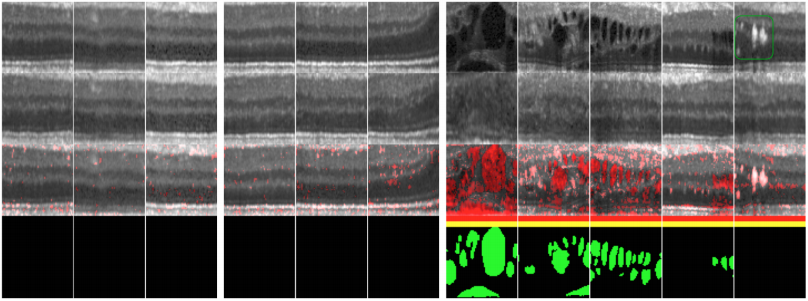
Pixel-level identification of anomalies on exemplary images. First row: Real input images. Second row: Corresponding images generated by the model triggered by our proposed mapping approach. Third row: Residual overlay. Red bar: Anomaly identification by residual score. Yellow bar: Anomaly identification by discrimination score. Bottom row: Pixel-level annotations of retinal fluid. First block and second block: Normal images extracted from OCT volumes of healthy cases in the training set and test set, respectively. Third block: Images extracted from diseased cases in the test set. Last column: Hyperreflective foci (within green box). (From Schlegl et al., 2017)
The second is a quantitative evaluation on anomaly detection accuracy of images based on both components (residual score , discrimination score of the anomaly score . The distributions for the anomalous images are distinguishable from the distribution of the normal images showing that both the residual and discriminator scores are relevant for classification. ROC curves of both components and an additional reference discrimination score based on a discrimination score proposed by Yeh et al., reveal that the novel discrimination score outperforms the reference discrimination score but the residual score has the highest impact on performance.
The final qualitative evaluation compares the AnoGAN against other models, namely adversarial convolutional autoencoder (aCAE), and a duplicate AnoGAN, denoted GANR, but using the reference discrimination score. The model with the worst performance is aCAE as it tends to over-adapt on anomalous images, followed by GANR which is only marginally worse than AnoGAN.
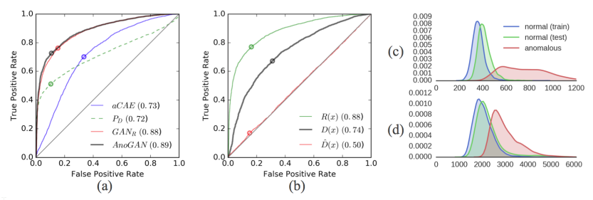
Image level anomaly detection performance and suitability evaluation. (a) Model comparison: ROC curves based on aCAE (blue), GANR (red), the proposed AnoGAN (black), or on the output PD of the trained discriminator (green). (b) Anomaly score components: ROC curves based on the residual score R(x) (green), the discrimination score D(x) (black), or the reference discrimination score Dˆ(x) (red). (c) Distribution of the residual score and (d) of the discrimination score, evaluated on normal images of the training set (blue) or test set (green), and on images extracted from diseased cases (red). (From Schlegel et al., 2017)
Application on Cancer Data
We used the technique presented in this paper to identify metastatic cancer in small image patches extracted from histopathologic scans of lymph node sections.
Data Preprocessing. Each patch is 64x64x3 and contains normalized valued between -1 and 1.
References and other papers
Unsupervised Representation Learning with Deep Convolutional Generative Adversarial Networks
Unsupervised Anomaly Detection with Generative Adversarial Networks to Guide Marker Discovery